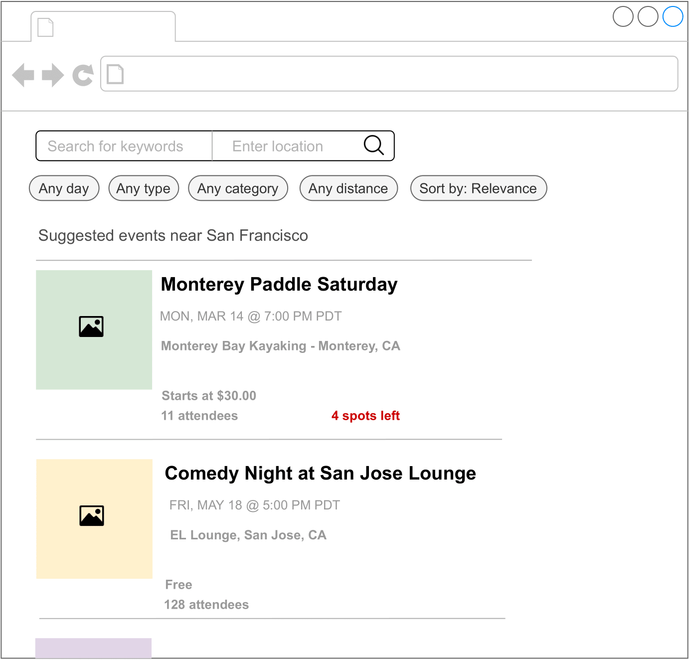
In this chapter, we design an event recommendation system similar to Eventbrite's. Eventbrite is a popular event management and ticketing marketplace which allows users to create, browse, and register events. A recommendation system personalizes the experience and displays events relevant to users.
Here is a typical interaction between a candidate and an interviewer.
Candidate: What is the business objective? Can I assume the main business objective is to increase ticket sales?
Interviewer: Yes, that sounds good.
Candidate: Besides attending an event, can users book hotels or restaurants on the platform?
Interviewer: For simplicity, let's assume only events are supported.
Candidate: An event is considered an ephemeral one-time occurrence item that only happens once, and then expires. Is this assumption correct?
Interviewer: That's an excellent observation.
Candidate: What event attributes are available? Can I assume we have access to the textual description of the event, price range, location, date and time, etc.?
Interviewer: Sure, those are fair assumptions.
Candidate: Do we have any annotated data?
Interviewer: We don't have a hand-labeled dataset. You can use event and user interaction data to construct the training dataset.
Candidate: Do we have access to the user's current location?
Interviewer: Yes. Since this problem focuses on a location-based recommendation system, let's assume users agree to share their location data.
Candidate: Can users become friends on the platform? Friendship information is valuable for building a personalized event recommendation system.
Interviewer: Good question. Yes, let's assume users can form friendships on our platform. A friendship is bidirectional, meaning if A is a friend of B, then B is also a friend of A.
Candidate: Can users invite others to events?
Interviewer: Yes.
Candidate: Can a user RSVP to an event?
Interviewer: For simplicity, let's assume only a registration option is available for an event.
Candidate: Are the events free or paid?
Interviewer: We need to support both.
Candidate: How many users and events are available?
Interviewer: We host around 1 million total events every month.
Candidate: How many daily active users visit the website/app?
Interviewer: Assume we have one million unique users per day.
Candidate: Since we are building a location-based event recommendation system, it's important to calculate the distance and travel time between two locations efficiently. Can we assume external APIs such as Google Maps API or other map services can be used to obtain such data?
Interviewer: Good point. Assume we can use third-party services to obtain location data.
Let's summarize the problem statement. We are asked to design an event recommendation system, which displays a personalized list of events to users. When an event is finished, users can no longer register for it. In addition to registering for events, users can invite others to events and form friendships. The training data should be constructed online from user interactions. The primary goal of this system is to increase total ticket sales.
Based on the requirements, the business objective is to increase ticket sales. One way to translate this into a well-defined ML objective is to maximize the number of event registrations.
The input to the system is a user, and the output is the top k events ranked by relevance to the user.
There are different ways to solve a recommendation problem:
Rule-based methods are good starting points to form a baseline. However, ML-based approaches usually lead to better outcomes. In this chapter, we reformulate the task into a ranking problem and use Learning to Rank (LTR) to solve it.
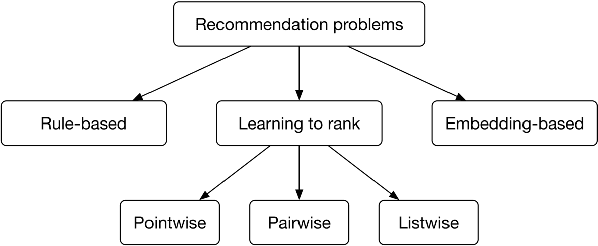
LTR is a class of algorithmic techniques that apply supervised machine learning to solve ranking problems. The ranking problem can be formally defined as: "having a query and a list of items, what is the optimal ordering of the items from most relevant to least relevant to the query?" There are generally three LTR approaches: pointwise, pairwise, and listwise. Let's briefly examine each. Note that a detailed explanation of these approaches is beyond the scope of this book. If you're interested in learning more about LTR, refer to [1] .
In this approach, we go over each item and predict the relevance between the query and the item, using classification or regression methods. Note that the score of one item is predicted independently of other items.

The final ranking is achieved by sorting the predicted relevance scores.
In this approach, the model takes two items and predicts which item is more relevant to the query.

Some of the most popular pairwise LTR algorithms are RankNet [2], LambdaRank [3], and LambdaMART [4].
Listwise approaches predict the optimal ordering of an entire list of items, given the query.

Some popular listwise LTR algorithms are SoftRank [5], ListNet [6], and AdaRank [7].
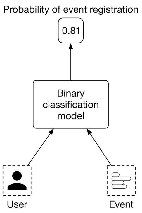
In general, pairwise and listwise approaches produce more accurate results, but they are more difficult to implement and train. For simplicity, we use the pointwise approach for this problem. In particular, we employ a binary classification model which takes a single event at a time and predicts the probability that the user will register for it. This approach is shown in Figure 7.6.
To engineer good features, we need first to understand the raw data available in the system. Since an event management platform is mainly centered around users and events, we assume the following data are available:
The user data schema is shown below.
| ID | Username | Age | Gender | City | Country | Language | Time zone |
|---|
Table 7.1: User data schema
Table 7.2 shows what the event data might look like.
| ID | Host User ID | Category/ Subcategory | Description | Price | Location | Date/Time |
|---|---|---|---|---|---|---|
| 1 | 5 | Music Concert | Dua Lipa Tour in Miami | 200-900 | American Airlines Arena Miami, FL | 09/18/2022 19:00-24:00 |
| 2 | 11 | Sports Basketball | Golden State Warriors vs. Milwaukee Bucks | 140-2500 | Chase Center SF, CA | 09/22/2022 17:00-19:00 |
| 3 | 7 | Art Theater | The Comedy and Magic of Robert Hall | Free | San Jose Improv San Jose, CA | 09/06/2022 18:00-19:30 |
Table 7.2: Event data
In Table 7.3, each row represents a friendship formed between two users, along with the timestamp of when it was formed
| User ID 1 | User ID 2 | Timestamp when friendship was formed |
|---|---|---|
| 28 | 3 | 1658451341 |
| 7 | 39 | 1659281720 |
| 11 | 25 | 1659312942 |
Table 7.3: Friendship data
Table 7.4 stores user interaction data, such as event registrations, invitations, and impressions. In practice, we may store interaction data in different databases, but for simplicity, we include them in a single table.
| User ID | Event ID | Interaction type | Interaction value | Location (lat, long) | Timestamp |
|---|---|---|---|---|---|
| 4 | 18 | Impression | - | 38.8951 -77.0364 | 1658450539 |
| 4 | 18 | Register | Confirmation number | 38.8951 -77.0364 | 1658451341 |
| 4 | 18 | Invite | User 9 | 41.9241 -89.0389 | 1658451365 |
Table 7.4: Interaction data
Event-based recommendations are more challenging than traditional recommendations. An event is fundamentally different from a movie or a book, as there is no consumption after the event ends. Events are typically short-lived, meaning the time is short between event creation and when it finishes. As a result, there are not many historical interactions available for a given event. For this reason, event-based recommendations are intrinsically cold-start and suffer from a constant new-item problem.
To overcome those issues, we put more effort into feature engineering to create as many meaningful features as possible. Due to space constraints, we will only discuss some of the most important features. In practice, the number of predictive features can be much higher. In this section, we create features related to each of the following categories:
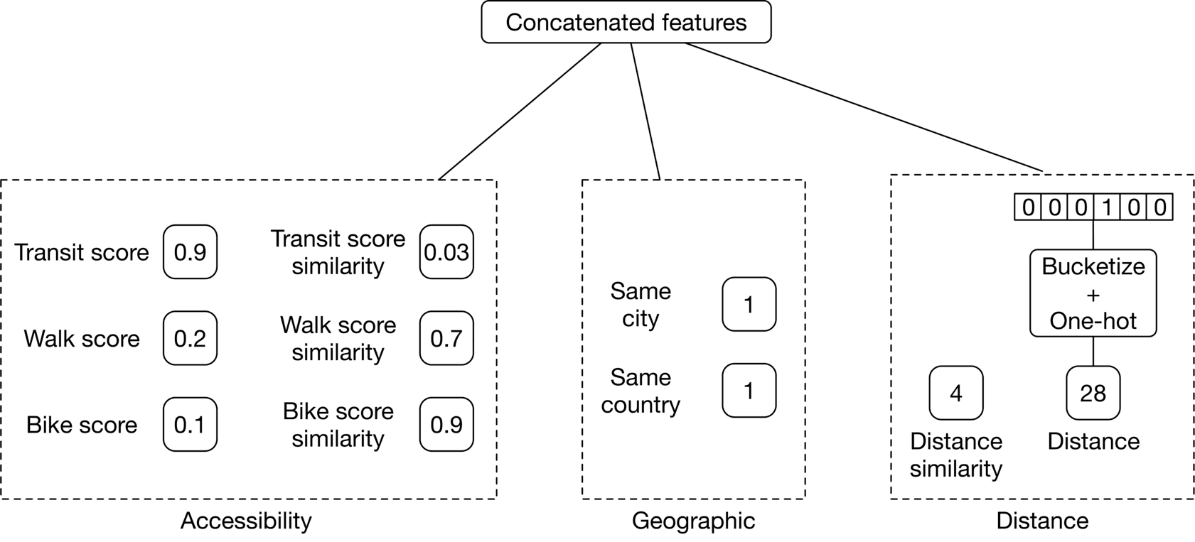
How accessible is the event's location?
The accessibility of an event's location is an important factor. For example, if an event is high up in hills far from public transportation, the commute may discourage users from attending. Let's create the following features to capture accessibility:
| Category | Walk score | Description |
|---|---|---|
| 1 | 90-100 | No car needed |
| 2 | 70-89 | Very walkable |
| 3 | 50-69 | Somewhat walkable |
| 4 | 25-49 | Car-dependent |
| 5 | 0-24 | Requires a car |
Table 7.5: Walk score categories
Is the event in the same country and city as the user?
A very important deciding factor for a user is whether the event is in the same country and city where they are located. The following two features can be created:
If the user's country is the same as the event's country, this feature is 1, otherwise 0
If the user's city is the same as the event's city, this feature is 1, otherwise 0
Is the user comfortable with the distance?
Some users may prefer events that are very close to their location, while others prefer events that are further away. We use the following features to capture this:
How convenient is the time remaining until an event?
Some users may plan events a few days in advance, while others don't. Let's create the following features to capture this:
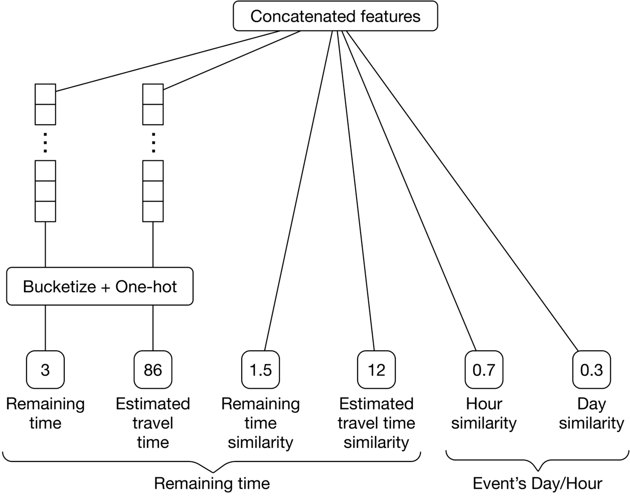
The remaining time until the event begins. This feature can be bucketized into different categories and one-hot encoded. For example:
Remaining time similarity: Difference between "remaining time" and average "remaining time" of events previously registered by the user.
The estimated travel time from the user's location to the event's location. This value will be obtained from external services and bucketized into categories.
Estimated travel time similarity: The difference between the estimated travel time to the event in question, and the average estimated travel time of events previously registered by the user.
Are the date and time convenient for the user?
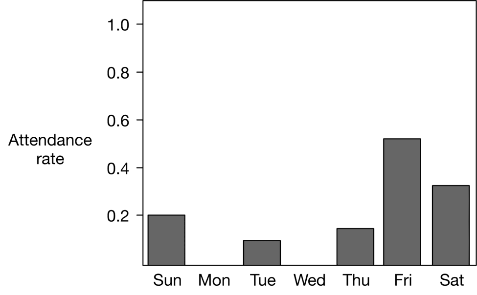
Some users may prefer events that occur at weekends, while others prefer weekdays. Some users prefer events in the morning, while others may prefer evening events. To capture a user's historical preferences for days of the week, we create a user profile. This user profile is a vector of size 7 , and each value counts the number of events the user attended on a particular day. By dividing these values by the total number of attended events, we get the historical rate of event attendance for each day of the week. Figure 7.8 shows the per-day distribution of a user's previously attended events. As we can see, this user has never attended an event on Monday or Wednesday, so displaying an event that occurs on Wednesday may not be a good recommendation for this user. Per-hour user profiles can be created using a similar approach. Similarly, we add day and hour similarity.
A summary of time-related features is shown in Figure 7.9
How many people are attending this event?
In general, users are more likely to register for an event if there are a lot of other attendees. Let's extract the following features to capture this:
Features related to attendance by friends
A user is more likely to register for an event if their friends are attending it. Here are some of the features we can use:
Is the user invited to this event by others?
Users are more likely to attend events to which they are invited. Some features that might be helpful are:
Is the event's host a friend of the user?
Users tend to attend events created by their friends. We create a binary feature to reflect this: if the event's host is the user's friend, this value is 1, otherwise, 0.
How often has the user attended previous events created by this host?
Some users are interested in following a particular host's events.
Age and gender
Some events are geared toward specific ages and genders. For example, "Women in Tech" and "Life lessons to excel in your 30 s" are examples of events that may be specific to certain demographic groups. We create two features to capture this:
Price of event:
The price of an event might affect the user's decision to register for it. Some features to use are:
How similar is this event's description to previously registered descriptions?
This indicates the user's interests, based on previously registered events. For example, if the word "concert" repeatedly appears in the descriptions of previous events, it may indicate the user is interested in concert events. To capture this, we create a feature that represents the similarity between the event's description and the descriptions of previously registered events by the user. To compute the similarity, the description is converted into a numerical vector using TF-ID, and similarity is calculated using cosine distance.
Note, this feature might be noisy as descriptions are manually provided by hosts. We can experiment by training our model with and without this feature, to measure its importance.
Figure shows an overview of user features, event features, and social-related features.
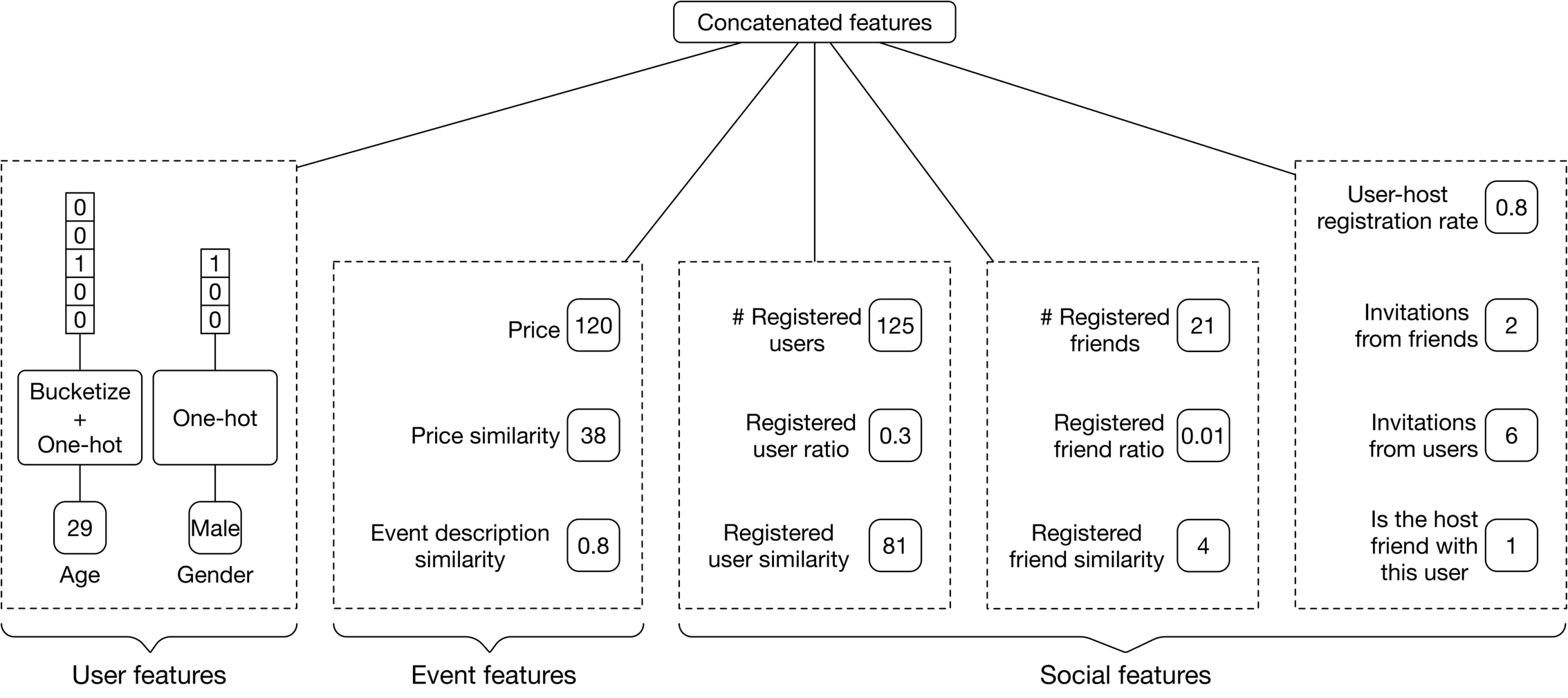
The features listed above are not exhaustive. There are lots of other predictive features that can be created in practice. For example, host-related features such as the host's popularity, user's search history, event's category, auto-generated event tags, etc. At an interview, it's not necessary to follow this section strictly. You can use it as a starting point and then discuss topics that are more relevant to the interviewer. Here are some potential talking points you might want to elaborate on:
Binary classification problems can be solved by various ML methods. Let's take a look at the following:
LR models the probability of a binary outcome by using a linear combination of one or multiple features. For the details of LR, refer to [10].
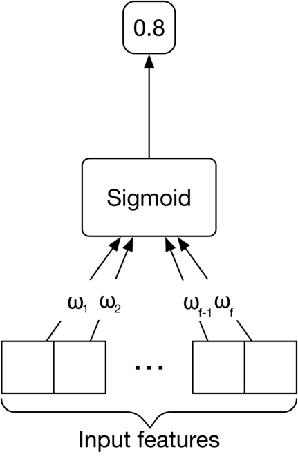
Let's see the pros and cons of LR.
Pros:
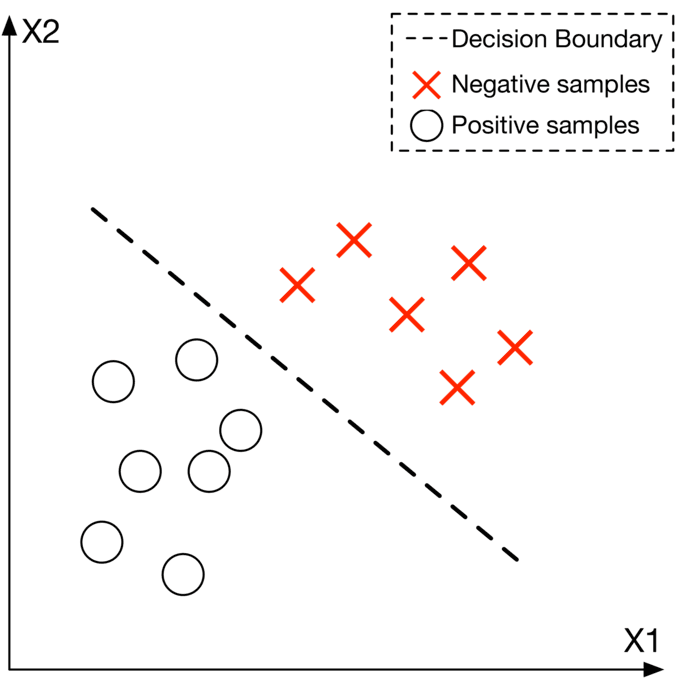
Cons:
In our system, the number of input features can be very large. Often, these features have complex and non-linear relations with the target variable (binary outcome). This complexity might be hard for LR to learn.
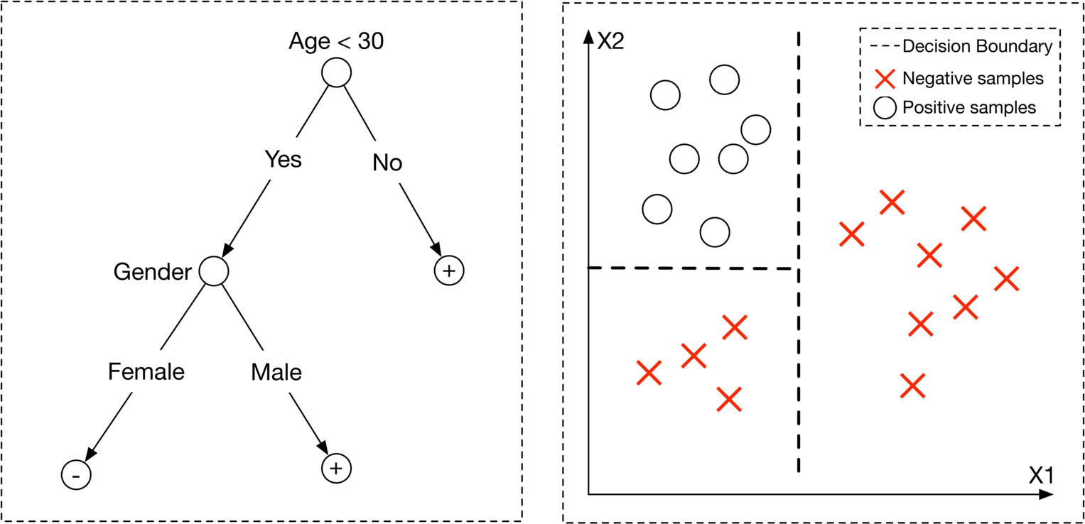
Decision trees are another class of learning methods that use a tree-like model of decisions and their possible consequences to make predictions. Figure 7.13 shows a simple decision tree with two features: age and gender. It also shows the corresponding decision boundary. Each leaf node in the decision tree indicates a binary outcome where "+" indicates the given input is classified as positive, and "-" means negative. To learn more about decision trees, refer to [11].
Pros:
Cons:
In practice, naive decision trees are rarely used. The reason is that they are too sensitive to variations of input data. To reduce the sensitivity of decision trees, two techniques are commonly used:
These two techniques are widely used across the tech industry. It's essential to understand how they work. Let's take a closer look.
Bagging is the ensemble learning method that trains a set of ML models in parallel, on multiple subsets of the training data. In bagging, the predictions of all these trained models are combined to make a final prediction. This significantly reduces the model's sensitivity to the change in data (variance).
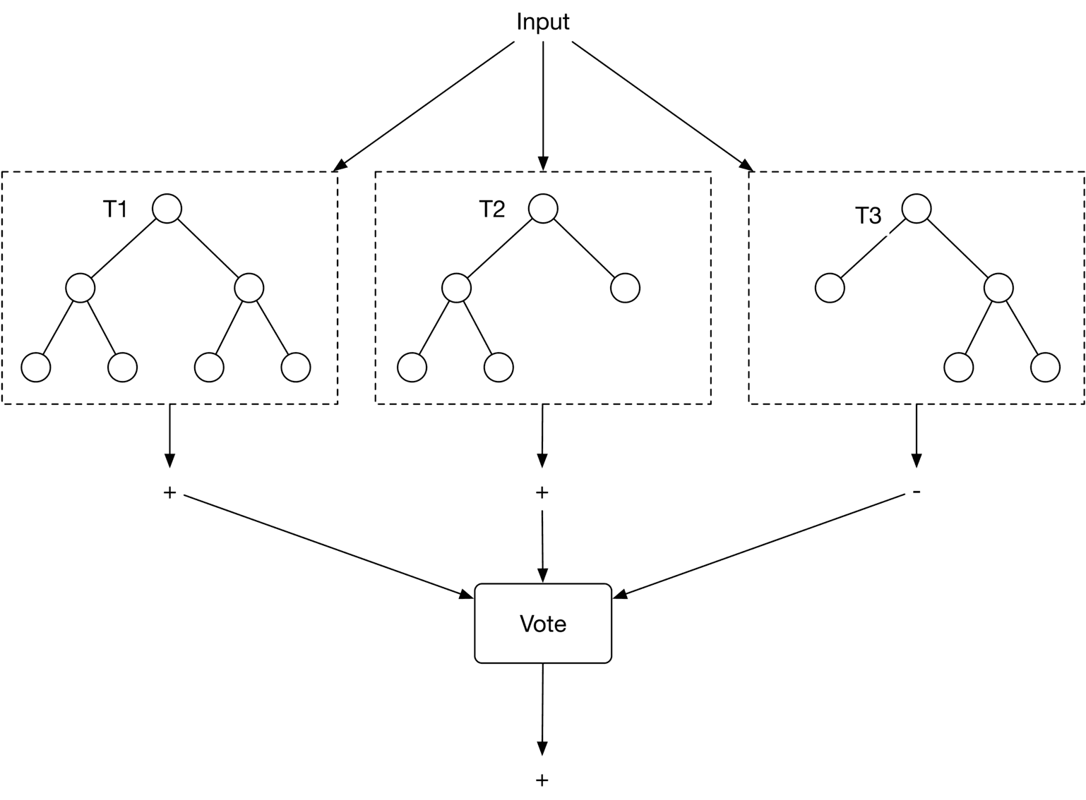
One example of bagging is the commonly used "random forest" model [12]. Random forest builds multiple decision trees in parallel during training, to reduce the model's sensitivity. To make a prediction, each decision tree independently predicts the output class (positive or negative) of the given input, and then a voting mechanism is used to combine these predictions to make a final prediction. Figure shows a random forest with three decision trees.
The bagging technique has the following advantages:
Despite its advantages, bagging is not helpful when the model faces underfitting (high bias). To overcome bagging’s drawbacks, let’s discuss another technique called boosting.
In ML, boosting involves training several weak classifiers sequentially to reduce prediction errors. The phrase "weak classifier" refers to a simple classifier that performs slightly better than random guesses. In boosting, multiple weak classifiers are converted into a single strong learning model. Figure shows an example of boosting.

Pros:
The boosting method is usually preferred over bagging in practice because bagging is not helpful in cases of bias, whereas boosting reduces the effect of both bias and variance.
Typical boosting-based decision trees are Adaboost [14], XGBoost [15], and Gradient boost [16]. They are commonly employed to train classification models.
GBDT is a commonly used tree-based model, utilizing GradientBoost to improve decision trees. Some variants of GBDT, such as XGBoost [15], have demonstrated strong performance in various ML competitions [17]. If you're interested in learning more about GBDT, refer to [18] [19].
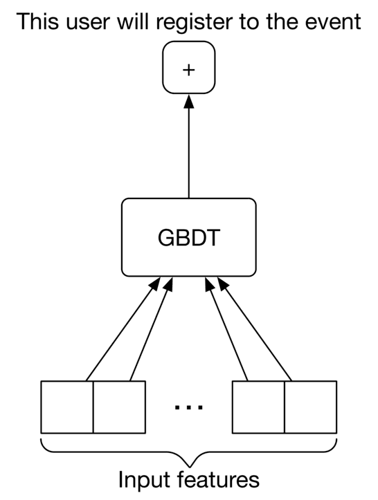
Here are the pros and cons of the GBDT model.
Pros:
Cons:
In our case, since the created features are structured data, GBDT or one of its variants such as XGBoost - is a good choice to experiment with.
A major drawback of GBDT is that it is unsuitable for continual learning. In an event recommendation system, new data continuously becomes available to the system, such as recent user interactions, registrations, new events, and even new users. In addition, users' tastes and interests may change over time. It is vital for a good event recommendation system to adapt itself to new data, continuously. Without the possibility of continual learning, it is very costly to retrain GBDT from scratch regularly. Next, we explore neural networks which overcome this limitation.
In an event recommendation system, we have many features that might not correlate linearly with the outcome. Learning these complex relationships is difficult. In addition, continual learning is necessary for adapting the model to new data.
NNs are great at solving those challenges. They are capable of learning complex tasks with non-linear decision boundaries. Additionally, NN models can be fine-tuned on new data very easily, making them ideal for continual learning. If you are unfamiliar with the details of NNs, you are encouraged to read [20].
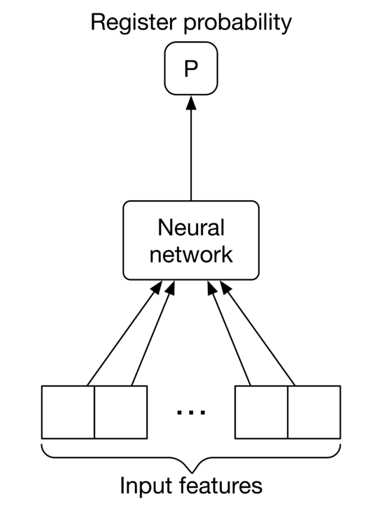
Let's see its pros and cons.
Pros
Cons
Picking the right model is challenging. We often need to experiment with different models to determine which works best. We can choose the right model based on various factors:
Once we have a baseline, we explore the possibility of building a better model with NNs. Neural networks are expected to work well here for the following reasons:
When designing a NN architecture, several hyperparameters must be considered, including the number of hidden layers, neurons in each layer, activation function, etc. These can be determined by employing hyperparameter tuning techniques. NN architectural details are not typically the main focus of ML system design interviews, since there is no systematic way to choose the right architecture.
Building training and evaluation datasets is an essential step in developing a model. For example, let's look at how we compute features and their labels.
To construct a single data point, we extract a user, event pair from the interaction data and compute the input features from the pair. We then label the data point with 1 if the user has registered for the event, and 0 if not.
![Image represents a tabular dataset seemingly used for training a machine learning model. The table has four columns. The first column, labeled '#', acts as a row identifier, with rows numbered '1' and '2'. The second column, labeled 'Extracted (user, event) features', contains a sequence of binary features (0s and 1s) for each row, representing extracted characteristics from user and event data. Row 1 shows features [1, 0, 1, 1, 0, 1], and row 2 shows features [0, 0, 0, 1, 1, 0]. Each feature likely corresponds to a specific attribute of the user or event. The third column is labeled 'Label', and contains a single binary value (0 or 1) for each row, representing the target variable or class label for the corresponding features. Row 1 has a label of '1', and row 2 has a label of '0'. The table structure suggests a supervised learning scenario where the model learns to predict the 'Label' based on the 'Extracted (user, event) features'.](images/img-bfe598c12671.png)
One issue we may face after constructing the dataset is class imbalance. The reason is that users may explore tens or hundreds of events before registering for one. Therefore, the number of negative user, event pairs is significantly higher than positive data points. We can use one of the following techniques to address the class imbalance issue:
Use focal loss or class-balanced loss to train the classifier
Undersample the majority class
Since the model is a binary classification model, we use a typical classification loss function such as binary cross-entropy to optimize the neural network model.
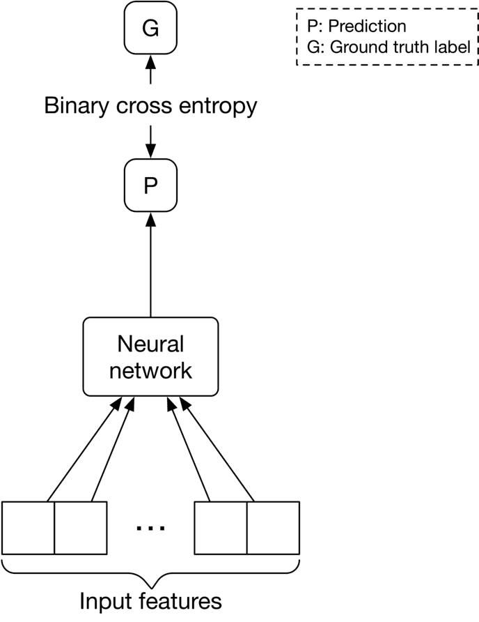
To evaluate the ranking system, we consider the following options.
Recall@k or Precision@k. These metrics are not good fits because they do not consider the ranking quality of the output.
MRR, nDCG, or mAP. These three metrics are commonly used to measure ranking quality. But which one is best?
MRR focuses on the rank of the first relevant item in the list, which is suitable in systems where only one relevant item is expected to be retrieved. However, in an event recommendation system, several recommended events may be relevant to the user. MRR is not a good fit.
nDCG works well when the relevance score between a user and an item is non-binary. In contrast, mAP works only when the relevance scores are binary. Since events are either relevant (a user registered for it) or irrelevant (a user saw the event but did not register), mAP is a better fit.
In our case, the business objective is to increase revenue by increasing ticket sales. To measure the impact of the system on revenue, let's explore the following metrics:
CTR. A ratio showing how often users who see recommended events go on to click on an event.
A high CTR shows our system is good at recommending events that users click on. Having more clicks generally means more event registrations.
However, relying only on CTR as the online metric may be insufficient. Some events are clickbait. Ideally, we would like to measure how relevant recommended events are for the user. This metric is called the conversion rate, which we discuss now.
Conversion rate. A ratio showing how often users who see recommended events go on to register for them. The formula is:
A high conversion rate indicates users register for recommended events more often. For example, a conversion rate of means that users, on average, register for 3 events out of every 10 recommended events.
Bookmark rate. A ratio showing how often users bookmark recommended events. This is based on the assumption that the platform allows users to save or bookmark an event.
Revenue lift. This is the increase in revenue as a result of event recommendations.
In this section, we propose an ML system design that can be used to serve requests. As Figure 7.20 shows, there are two main pipelines in the design:
Online learning pipeline
Prediction pipeline
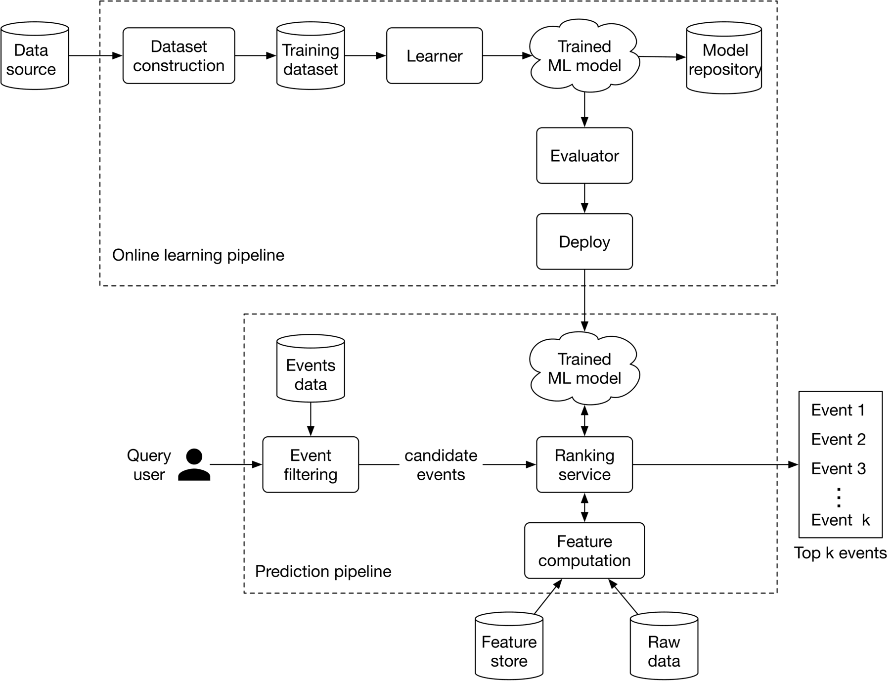
As described earlier, event recommendations are intrinsically cold-start and suffer from a constant new-item problem. Consequently, the model must be continuously fine-tuned to adapt to new data. This pipeline is responsible for continuously training new models by incorporating new data, evaluating the trained models, and deploying them.
The prediction pipeline is responsible for predicting the top most relevant events to a given user. Let's discuss some of the most important components of the prediction pipeline.
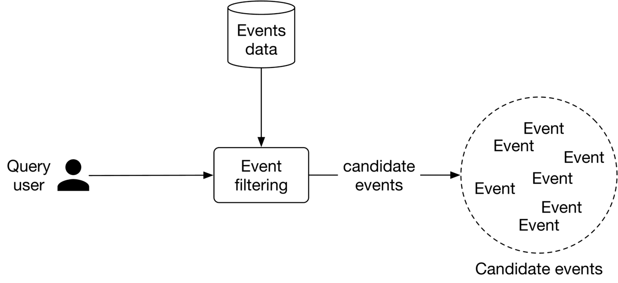
The event filtering component takes the query user as input and narrows down the events from 1 million to a small subset of events. This is based upon simple rules, such as event locations, or other types of user filters. For example, if a user adds a “concerts only” filter, the component quickly narrows down the list to a subset of candidate events. Since these types of filters are common in event recommendation systems, they can be used to significantly reduce our search space from potentially millions of events, to hundreds of candidate events.
This service takes the user and candidate events produced by the filtering component as input, computes features for each user, event pair, sorts the events based on the probabilities predicted by the model, and outputs a ranked list of top most relevant events to the user.
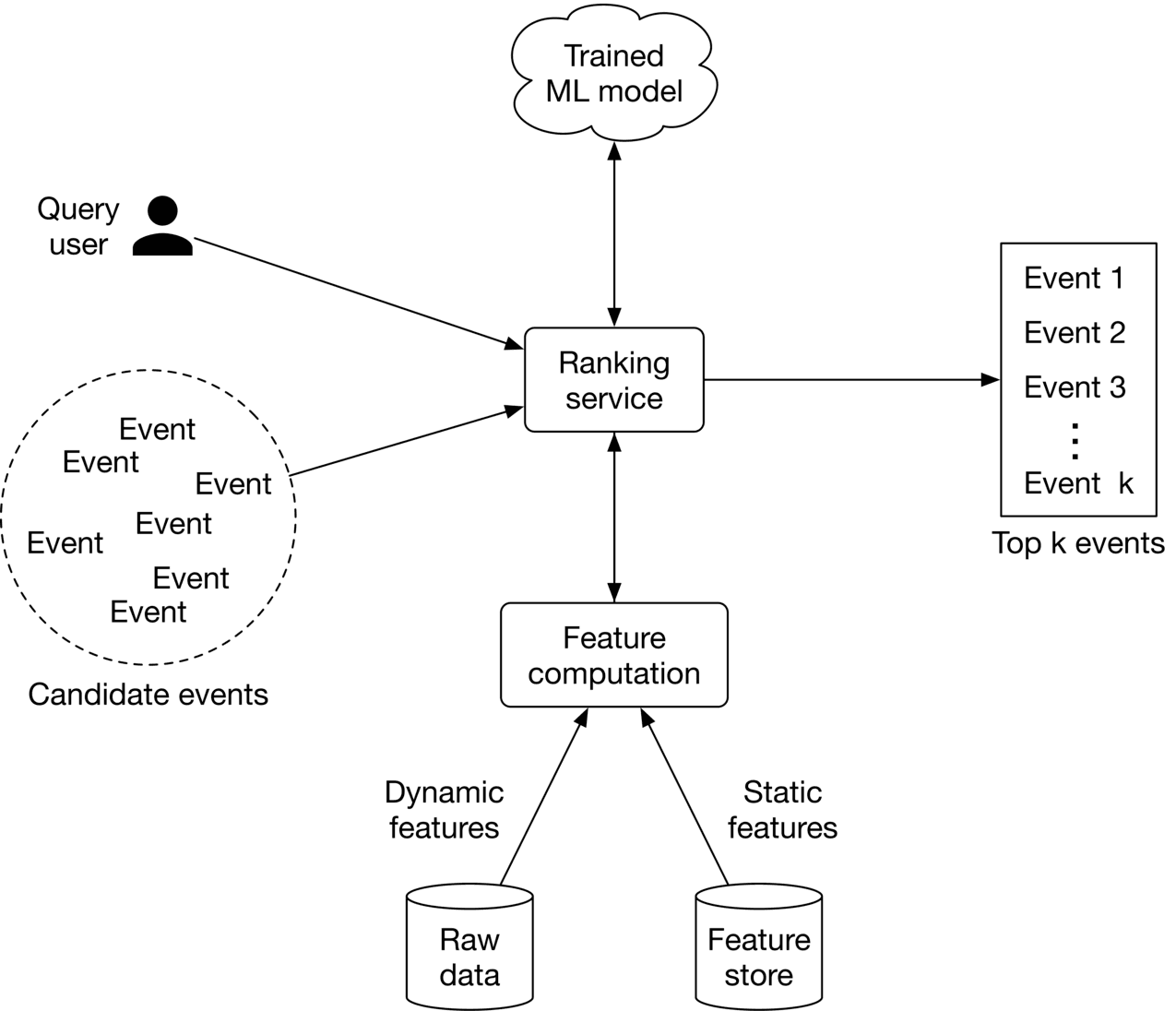
Ranking service interacts with the feature computation component responsible for computing features that the model expects. Static features are obtained from a feature store, while dynamic features are computed in real-time from the raw data.
If there is extra time at the end of the interview, here are some additional talking points: