Recommendation systems play a key role in video and music streaming services. For example, YouTube recommends videos a user may like, Netflix recommends movies a user may enjoy watching, and Spotify recommends music to users.
In this chapter, we design a video recommendation system similar to YouTube's [1]. The system recommends videos on the user's homepage based on their profile, previous interactions, etc.
Recommendation systems are often very complex in design, and a good amount of engineering effort is required to develop an efficient and scalable system. Don't worry, though; no one expects you to build the perfect system in a 45 -minute interview. The interviewer is primarily interested in observing your thought process, communication skills, ability to design ML systems, and ability to discuss trade-offs.
Here is a typical interaction between a candidate and an interviewer.
Candidate: Can I assume the business objective of building a video recommendation system is to increase user engagement?
Interview: That’s correct.
Candidate: Does the system recommend similar videos to a video a user is watching right now? Or does it show a personalized list of videos on the user’s homepage?
Interviewer: This is a homepage video recommendation system, which recommends personalized videos to users when they load the homepage.
Candidate: Since YouTube is a global service, can I assume users are located worldwide and videos are in different languages?
Interviewer: That’s a fair assumption.
Candidate: Can I assume we can construct the dataset based on user interactions with video content?
Interviewer: Yes, that sounds good.
Candidate: Can a user group videos together by creating playlists? Playlists can be informative for the ML model during the learning phase.
Interviewer: For the sake of simplicity, let’s assume the playlist feature does not exist.
Candidate: How many videos are available on the platform?
Interviewer: We have about 10 billion videos.
Candidate: How fast should the system recommend videos to a user? Can I assume the recommendation should not take more than 200 milliseconds?
Interviewer: That sounds good.
Let’s summarize the problem statement. We are asked to design a homepage video recommendation system. The business objective is to increase user engagement. Each time a user loads the homepage, the system recommends the most engaging videos. Users are located worldwide, and videos can be in different languages. There are approximately 10 billion videos on the platform, and recommendations should be served quickly.
The business objective of the system is to increase user engagement. There are several options available for translating business objectives into well-defined ML objectives. We will examine some of them and discuss their trade-offs.
Maximize the number of user clicks. A video recommendation system can be designed to maximize user clicks. However, this objective has one major drawback. The model may recommend videos that are so-called "clickbait", meaning the title and thumbnail image look compelling, but the video's content may be boring, irrelevant, or even misleading. Clickbait videos reduce user satisfaction and engagement over time.
Maximize the number of completed videos. The system could also recommend videos users will likely watch to completion. A major problem with this objective is that the model may recommend shorter videos that are quicker to watch.
Maximize total watch time. This objective produces recommendations that users spend more time watching.
Maximize the number of relevant videos. This objective produces recommendations that are relevant to users. Engineers or product managers can define relevance based on some rules. Such rules can be based on implicit and explicit user reactions. For example, one definition could state a video is relevant if a user explicitly presses the "like" button or watches at least half of it. Once we define relevance, we can construct a dataset and train a model to predict the relevance score between a user and a video.
In this system, we choose the final objective as the ML objective because we have more control over what signals to use. In addition, it does not have the shortcomings of the other options described earlier.
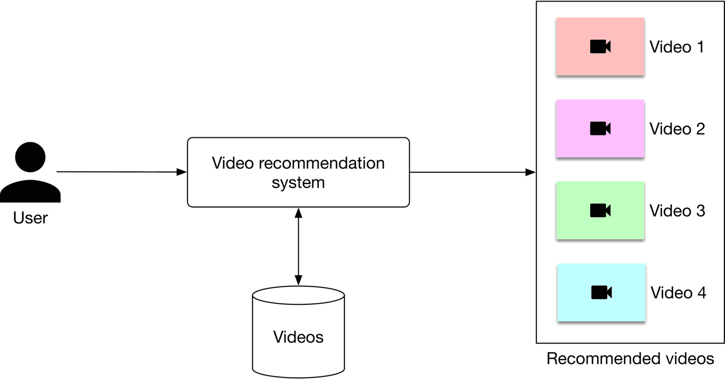
As Figure 6.2 shows, a video recommendation system takes a user as input and outputs a ranked list of videos sorted by their relevance scores.
In this section, we examine three common types of personalized recommendation systems.
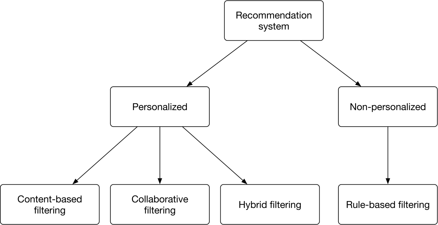
Let’s examine each type in more detail.
This technique uses video features to recommend new videos similar to those a user found relevant in the past. For example, if a user previously engaged with many ski videos, this method will suggest more ski videos. Figure shows an example.
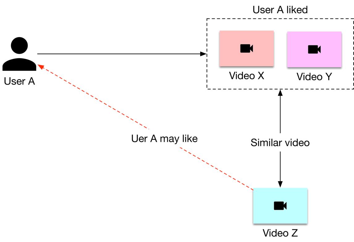
Here is an explanation of the diagram.
Content-based filtering has pros and cons.
Pros:
Cons:
CF uses user-user similarities (user-based CF) or video-video similarities (item-based CF) to recommend new videos. CF works with the intuitive idea that similar users are interested in similar videos. You can see a user-based CF example in Figure 6.5.
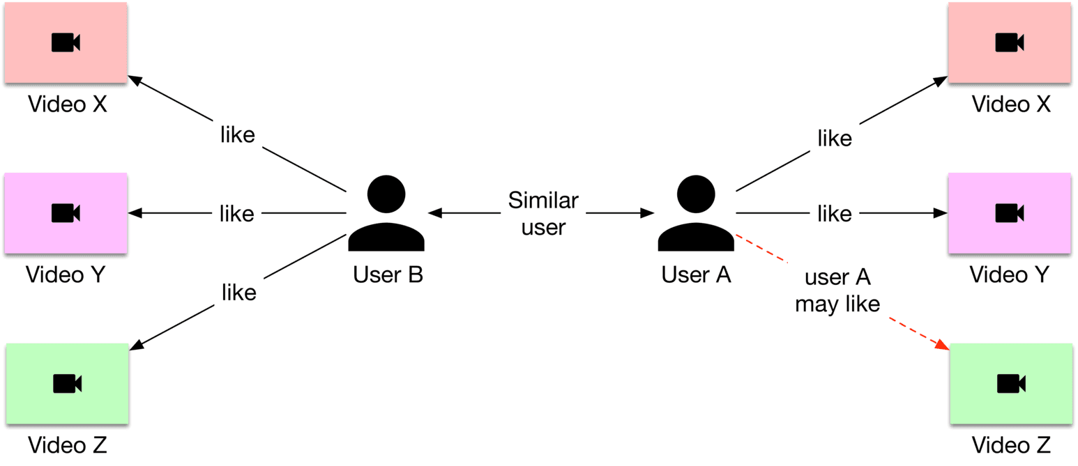
Let's explain the diagram. The goal is to recommend a new video to user A.
A major difference between content-based filtering and CF filtering is that CF filtering does not use video features and relies exclusively upon users' historical interactions to make recommendations. Let's see the pros and cons of CF filtering.
Pros:
Cons:
| Contentbased filtering | Collaborative filtering | |
|---|---|---|
| Handle new videos | ✓ | ✘ |
| Discover new interest areas | ✘ | ✓ |
| No domain knowledge necessary | ✘ | ✓ |
| Efficiency | ✘ | ✓ |
Table 6.1: Comparison between content-based filtering and CF
A comparison of the two types of filtering is shown in Table 6.1. As you see, the two methods are complementary.
Hybrid filtering uses both CF and content-based filtering. As Figure 6.6 shows, hybrid filtering combines CF-based and content-based recommenders sequentially, or in parallel. In practice, companies usually use sequential hybrid filtering [2].
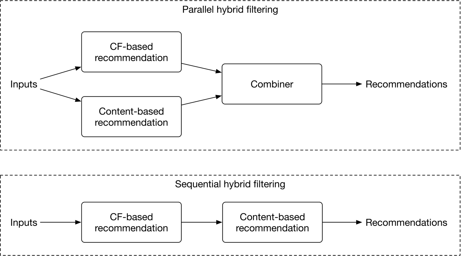
This approach leads to better recommendations because it uses two data sources: the user's historical interactions and video features. Video features allow the system to recommend relevant videos based on videos the user engaged with in the past, and CF-based filtering helps users to discover new areas of interest.
Many companies use hybrid filtering to make better recommendations. For example, a paper published by Google [2] describes how YouTube employs a CF-based model as the first stage (candidate generator), followed by a content-based model as the second stage, to recommend videos. Due to the advantages of hybrid filtering, we choose this option.
We have the following data available:
Video data contains raw video files and their associated metadata, such as video ID, video length, video title, etc. Some of these attributes are provided explicitly by video uploaders, and others can be implicitly determined by the system, such as the video length.
| Video ID | Length | Manual tags | Manual title | Likes | Views | Language |
|---|---|---|---|---|---|---|
| 1 | 28 | Dog, Family | Our lovely dog playing! | 138 | 5300 | English |
| 2 | 300 | Car, Oil | How to change your car oil? | 5 | 250 | Spanish |
| 3 | 3600 | Ouli, Vlog | Honeymoon to Bali | 2200 | 255K | Arabic |
Table 6.2: Video metadata
The following simple schema represents user data.
| ID | Username | Age | Gender | City | Country | Language | Time zone |
|---|
Table 6.3: User data schema
The user-video interaction data consists of various user interactions with the videos, including likes, clicks, impressions, and past searches. Interactions are recorded along with other contextual information, such as location and timestamp. The following table shows how user-video interactions are stored.
| User ID | Video ID | Interaction type | Interaction value | Location (lat, long) | Timestamp |
|---|---|---|---|---|---|
| 4 | 18 | Like | - | 38.8951 -77.0364 | 1658451361 |
| 2 | 18 | Impression | 8 seconds | 38.8951 -77.0364 | 1658451841 |
| 2 | 6 | Watch | 46 minutes | 41.9241 -89.0389 | 1658822820 |
| 6 | 9 | Click | - | 22.7531 47.9642 | 1658832118 |
| 9 | - | Search | Basics of clustering | 22.7531 47.9642 | 1659259402 |
| 8 | 6 | Comment | Amazing video. Thanks | 37.5189 122.6405 | 1659244197 |
Table 6.4: User-video interaction data
The ML system is required to predict videos that are relevant to users. Let's engineer features to help the system make informed predictions.
Some important video features include:
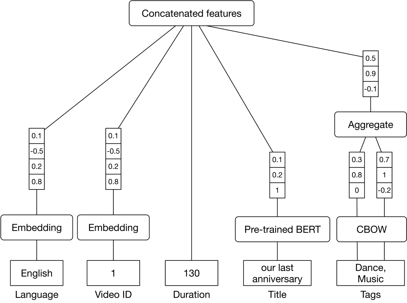
The IDs are categorical data. To represent them by numerical vectors, we use an embedding layer, and the embedding layer is learned during model training.
This defines approximately how long the video lasts from start to finish. This information is important since some users may prefer shorter videos, while others prefer longer videos.
The language used in a video is an important feature. This is because users naturally prefer particular languages. Since language is a categorical variable and takes on a finite set of discrete values, we use an embedding layer to represent it.
Titles and tags are used to describe a video. They are either provided manually by the uploader or are implicitly predicted by standalone ML models. The titles and tags of a video are valuable predictors. For example, a video titled "how to make pizza" indicates the video is related to pizza and cooking.
How to prepare it? For tags, we use a lightweight pre-trained model, such as CBOW [3], to map them into feature vectors.
For the title, we map it into a feature vector using a context-aware word embedding model, such as a pre-trained BERT [4].
Figure 6.7 shows an overview of video feature preparation.
We categorize user features into the following buckets:
An overview of user demographic features is shown in Figure 6.8.
![Image represents a data preprocessing pipeline for a machine learning model. The topmost box, 'Concatenated features,' represents the final output of the pipeline, a combined feature vector. This vector is formed by concatenating the outputs of six separate feature processing branches. Each branch processes a single feature: User ID (embedding resulting in a single value '1'), Age (bucketized and one-hot encoded resulting in the value '28'), Gender (one-hot encoded as 'Female'), Language (embedding resulting in 'English'), City (embedding resulting in 'SF'), and Country (embedding resulting in 'USA'). Each branch initially receives a vector of numerical values (e.g., [0.1, 0.9, 0.2, 0.7, 1] for User ID). These vectors are then processed using different techniques: embedding (for User ID, Language, City, and Country), which transforms categorical data into numerical vectors, and bucketization plus one-hot encoding (for Age), which transforms numerical data into categorical representations. The final output of each branch is then concatenated to form the 'Concatenated features' vector used as input to the machine learning model (not shown).](images/img-d19f1e785f2c.png)
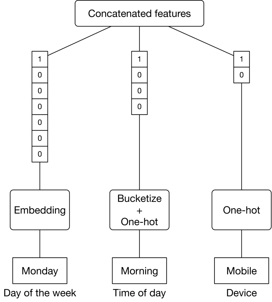
Here are a few important features for capturing contextual information:
User historical interactions play an important role in understanding user interests. A few features related to historical interactions are:
Search history
Why is it important?
Previous searches indicate what the user looked for in the past, and past behavior is often an indicator of future behavior.
How to prepare it?
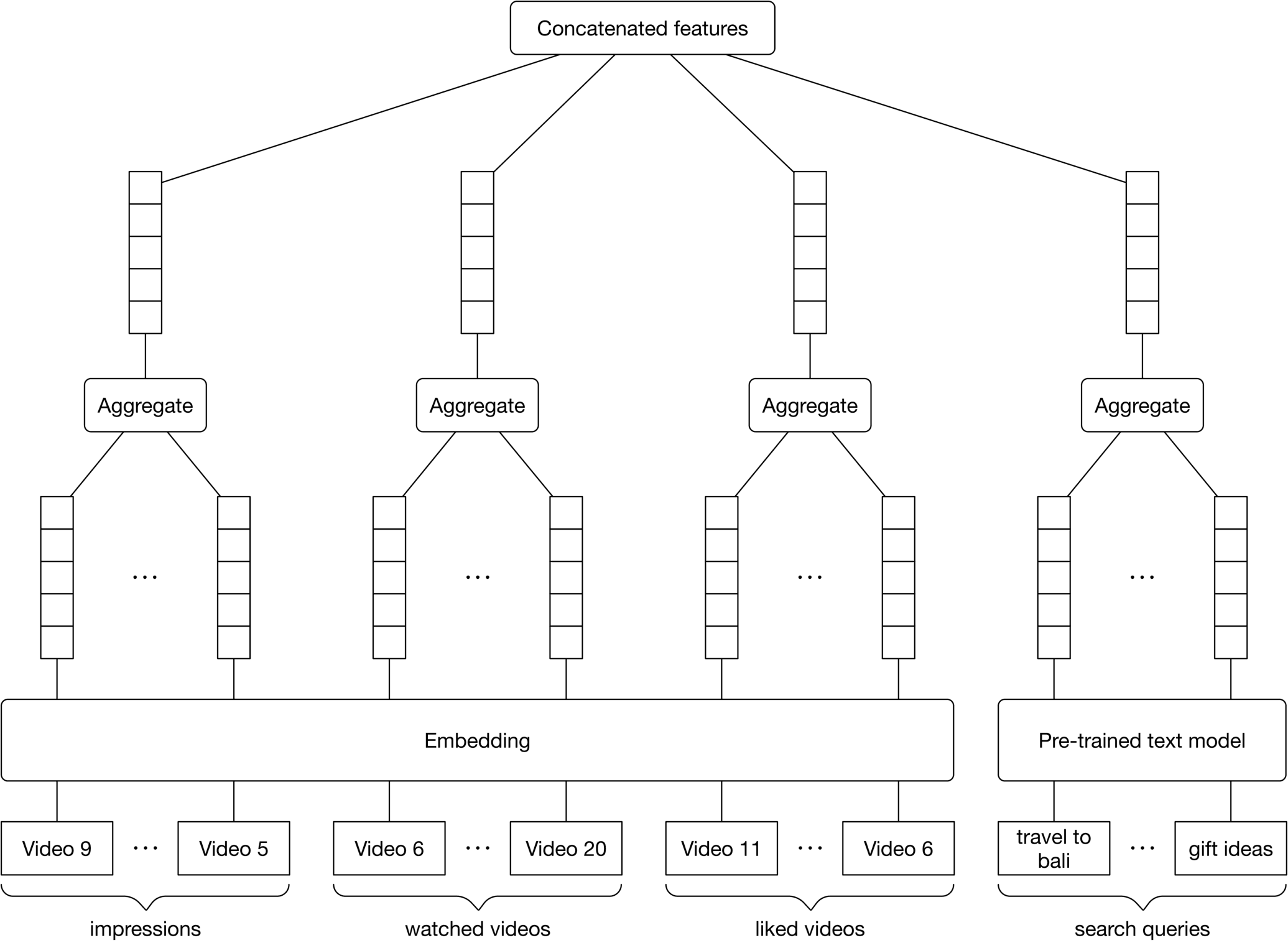
Use a pre-trained word embedding model, such as BERT, to map each search query into an embedding vector. Note that a user's search history is a variable-sized list of textual queries. To create a fixed-size feature vector summarizing all the search queries, we average the query embeddings.
Liked videos
Why is it important?
The videos a user liked previously can be helpful in determining which type of content they're interested in.
How to prepare it?
Video IDs are mapped into embedding vectors using the embedding layer. Similarly to search history, we average liked embeddings to get a fixed-size vector of liked videos.
Watched videos and impressions
The feature engineering process for “watched videos" and “impressions" is very similar to what we did for liked videos. So, we won’t repeat it.
Figure 6.10 summarizes features related to user-video interactions.
In this section, we examine two embedding-based models that are typically employed in CF-based or content-based recommenders:
To understand the matrix factorization model, it is important to know what a feedback matrix is.
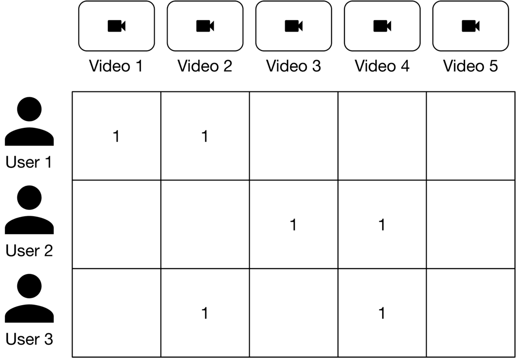
Also called a utility matrix, this is a matrix that represents users' opinions about videos. Figure 6.11 shows a binary user-video feedback matrix where each row represents a user, and each column represents a video. The entries in the matrix specify the user's opinion to 1 as "observed" or "positive."
How can we determine whether a user finds a recommended video relevant? We have three options:
Explicit feedback. A feedback matrix is built based on interactions that explicitly indicate a user's opinion about a video, such as likes and shares. Explicit feedback reflects a user's opinion accurately as users explicitly expressed their interest in a video. This option, however, has one major drawback: the matrix is sparse since only a small fraction of users provide explicit feedback. Sparsity makes ML models difficult to train.
Implicit feedback. This option uses interactions that implicitly indicate a user's opinion about a video, such as "clicks" or "watch time". With implicit feedback, more data points are available, resulting in a better model after training. Its main disadvantage is that it does not directly reflect users' opinions and might be noisy.
Combination of explicit and implicit feedback. This option combines explicit and implicit feedback using heuristics.
What is the best option for building our feedback matrix?
Since the model needs to learn the values of the feedback matrix, it's important to build the matrix that aligns well with the ML objective we chose earlier.
In our case, the ML objective is to maximize relevancy, where relevancy is defined as the combination of explicit and implicit feedback. As such, the final option of combining explicit and implicit feedback is the best choice.
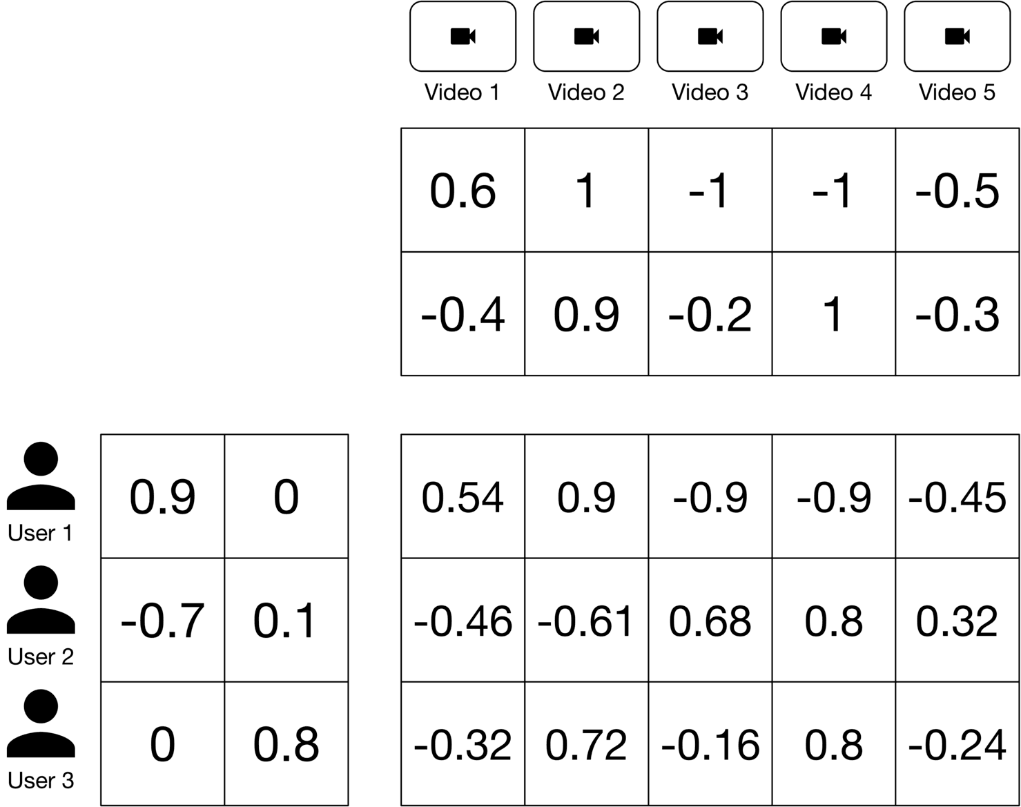
Matrix factorization is a simple embedding model. The algorithm decomposes the user-video feedback matrix into the product of two lower-dimensional matrices. One lower-dimensional matrix represents user embeddings, and the other represents video embeddings. In other words, the model learns to map each user into an embedding vector and each video into an embedding vector, such that their distance represents their relevance. Figure shows how a feedback matrix is decomposed into user and video embeddings.
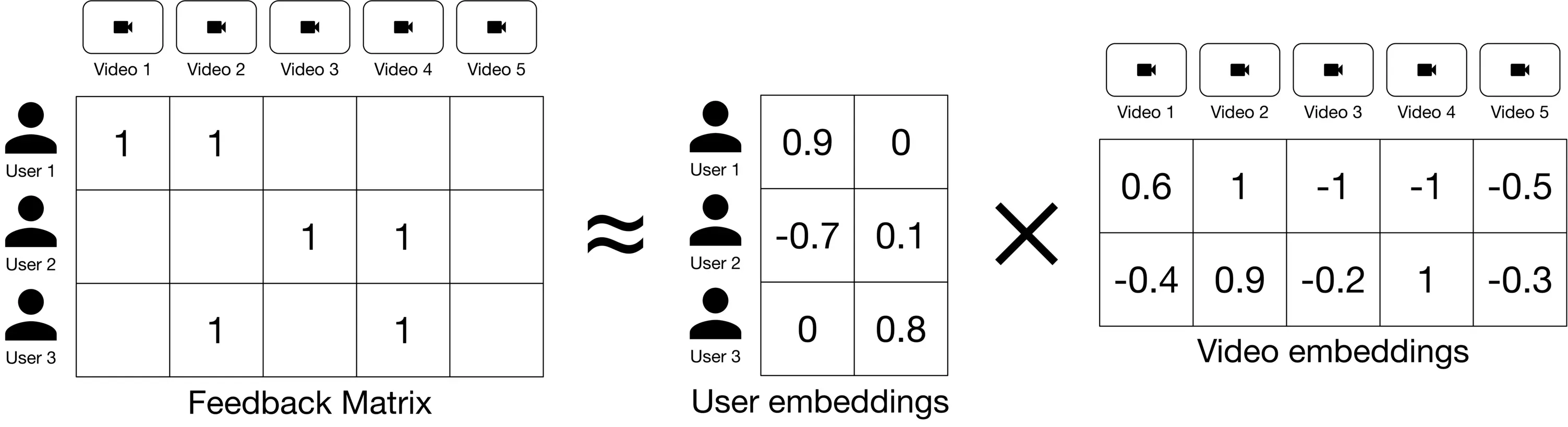
As part of training, we aim to produce user and video embedding matrices so that their product is a good approximation of the feedback matrix (Figure 6.13.)
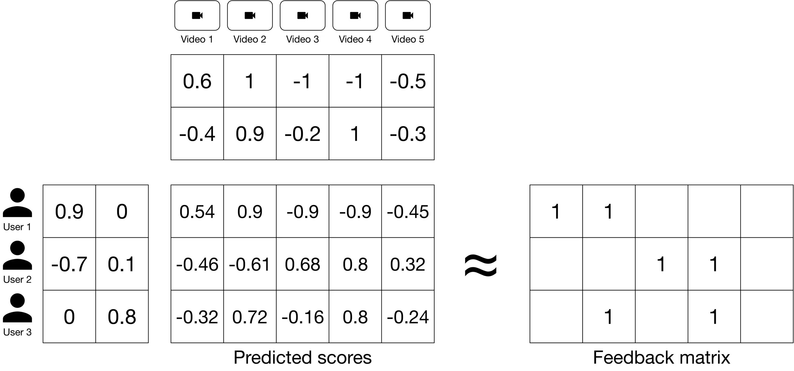
To learn these embeddings, matrix factorization first randomly initializes two embedding matrices, then iteratively optimizes the embeddings to decrease the loss between the "Predicted scores matrix" and the "Feedback matrix". Loss function selection is an important consideration. Let's explore a few options:
Squared distance over observed user, video pairs
This loss function measures the sum of the squared distances over all pairs of observed (non-zero values) entries in the feedback matrix. This is shown in Figure 6.14.
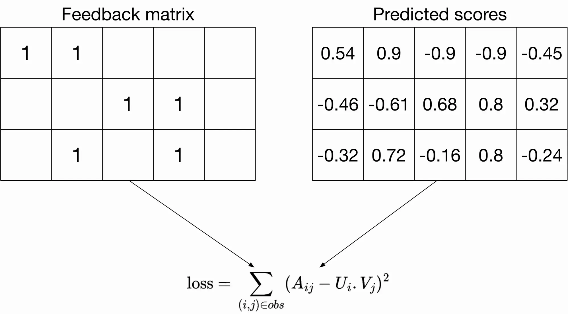
refers to the entry with row and column in the feedback matrix, is the embedding of user is the embedding of video , and the summation is over the observed pairs only.
Only summing over observed pairs leads to poor embeddings because the loss function doesn't penalize the model for bad predictions on unobserved pairs. For example, embedding matrices of all ones would have a zero loss on the training data. However, those embeddings may not work well for unseen user, video pairs.
Squared distance over both observed and unobserved user, video pairs This loss function treats unobserved pairs as negative data points and assigns a zero to them in the feedback matrix. As Figure 6.15 shows, the loss computes the sum of the squared distances over all entries in the feedback matrix.
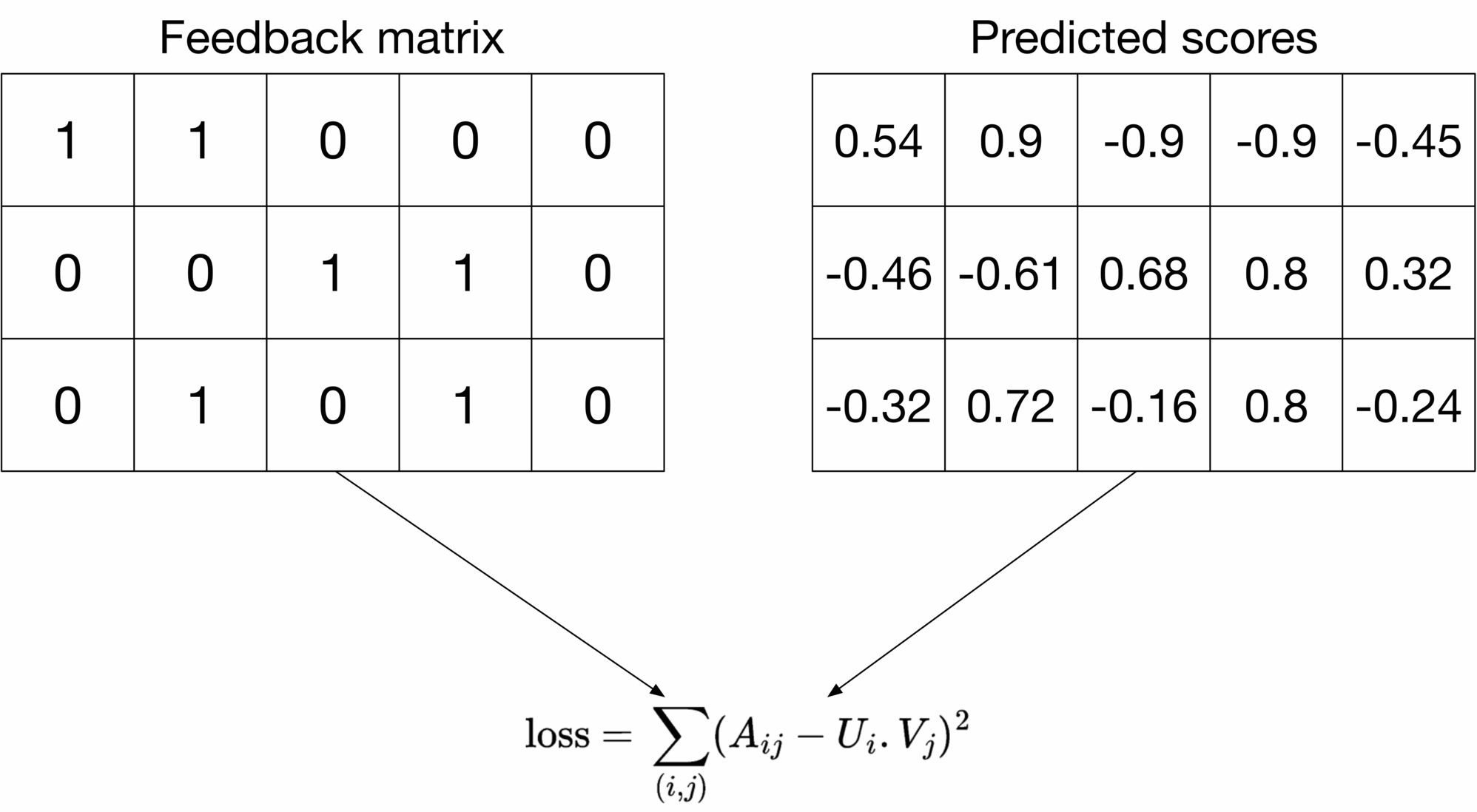
This loss function addresses the previous issue by penalizing bad predictions for unobserved entries. However, this loss has a major drawback. The feedback matrix is usually sparse (lots of unobserved pairs), so unobserved pairs dominate observed pairs during training. This results in predictions that are mostly close to zero. This is not desirable and leads to poor generalization performance on unseen user, video pairs.
A weighted combination of squared distance over observed and unobserved pairs
To overcome the drawbacks of the loss functions described earlier, we opt for weighted combinations of both.
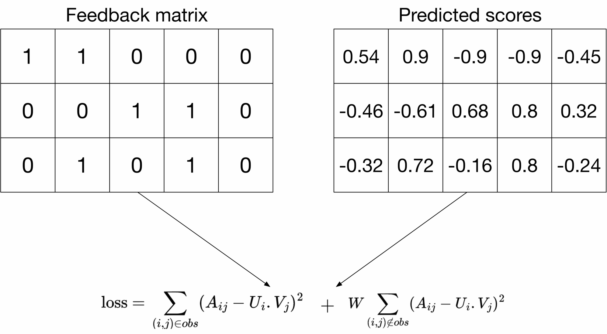
The first summation in the loss formula calculates the loss on the observed pairs, and the second summation calculates the loss on unobserved pairs. is a hyperparameter that weighs the two summations. It ensures one does not dominate the other in the training phase. This loss function with a properly tuned works well in practice [5]. We choose this loss function for the system.
To train an ML model, an optimization algorithm is required. Two commonly used optimization algorithms in matrix factorization are:
Fix the other embedding matrix (V), and optimize the embedding matrix (U)
To predict the relevance between an arbitrary user and a candidate video, we calculate the similarity between their embeddings using a similarity measure, such as a dot product. For example, as shown in Figure 6.17, the relevance score between user 2 and video 5 is .
![Image represents a simplified illustration of a dot product calculation. Two data sources are shown: 'User 2,' represented by a person icon, and 'Video 5,' represented by a video camera icon. Each source is associated with a two-element vector; User 2 has the vector [-0.7, 0.1], and Video 5 has the vector [-0.5, -0.3]. Arrows indicate that these vectors are inputs to a 'dot product' calculation. The calculation itself is explicitly shown as `dot product = (-0.7) * (-0.5) + (0.1) * (-0.3) = 0.32`, demonstrating the element-wise multiplication and summation that defines the dot product. The result, 0.32, is implicitly the output of the dot product operation. The diagram visually depicts the process of combining data from two different sources (user and video) using a vector dot product to obtain a single scalar value.](images/img-b82ef4d3b07a.png)
Figure 6.18 shows the predicted scores for all the user, video pairs. The system returns recommended videos based on relevance scores.
| Reminder |
|---|
| Since matrix factorization uses user-video interactions only, it is commonly used in collaborative filtering. |
Before wrapping up matrix factorization, let’s discuss the pros and cons of this model.
Pros:
Cons:
Let's see how two-tower neural networks address the shortcomings of matrix factorization.
A two-tower neural network comprises two encoder towers: the user tower and the video tower. The user encoder takes user features as input and maps them to an embedding vector (user embedding). The video encoder takes video features as input and maps them into an embedding vector (video embedding). The distance between their embeddings in the shared embedding space represents their relevance.
Figure 6.19 shows the two-tower architecture. In contrast to matrix factorization, twotower architectures are flexible enough to incorporate all kinds of features to better capture the user's specific interests.
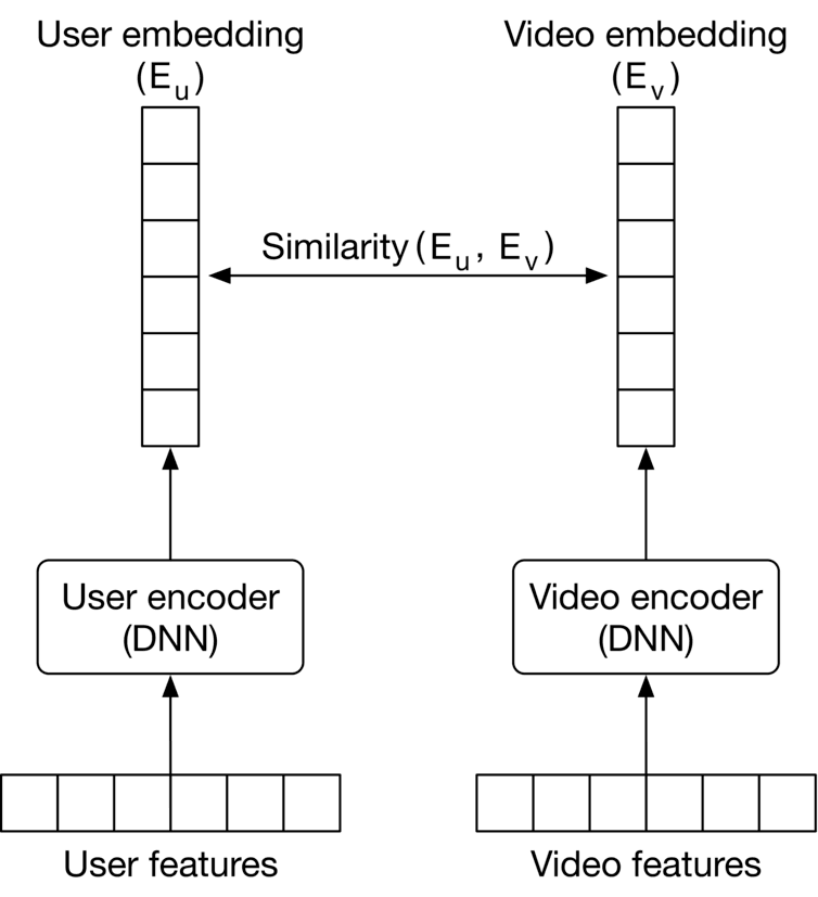
We construct the dataset by extracting features from different user, video pairs and labeling them as positive or negative based on the user's feedback. For example, we label a pair as "positive" if the user explicitly liked the video, or watched at least half of it.
To construct negative data points, we can either choose random videos which are not relevant or choose those the user explicitly disliked by pressing the dislike button. Figure 6.20 shows an example of the constructed data points.
![Image represents a tabular dataset used for training a machine learning model. The table is divided into four columns: a serial number column '#' identifying each data instance; a column labeled 'User-related features' containing a vector of seven numerical features for each user; a column labeled 'Video-related features' containing another vector of seven numerical features for each video; and a final column labeled 'Label' indicating the class of each data instance (1 for positive, 0 for negative). Each row represents a single data point, showing the user features, video features, and the corresponding label. For instance, row 1 shows user features [0, 0, 1, 0.7, -0.6, 0, 0], video features [0, 1, 0, 0.9, 0.9, 1], and a positive label (1). Row 2 similarly presents another data point with different feature values and a negative label (0). The features are likely used as input to a machine learning model to predict the label (positive or negative sentiment, for example).](images/img-2b4871038173.png)
Note, users usually only find a small fraction of videos relevant. While constructing training data, this leads to an imbalanced dataset where there are many more negative than positive pairs. Training a model on an imbalanced dataset is problematic. We can use the techniques described in Chapter 1 Introduction and Overview, to address the data imbalance issue.
Since the two-tower neural network is trained to predict binary labels, the problem can be categorized as a classification task. We use a typical classification loss function, such as cross-entropy, to optimize the encoders during training. This process is shown in Figure 6.21
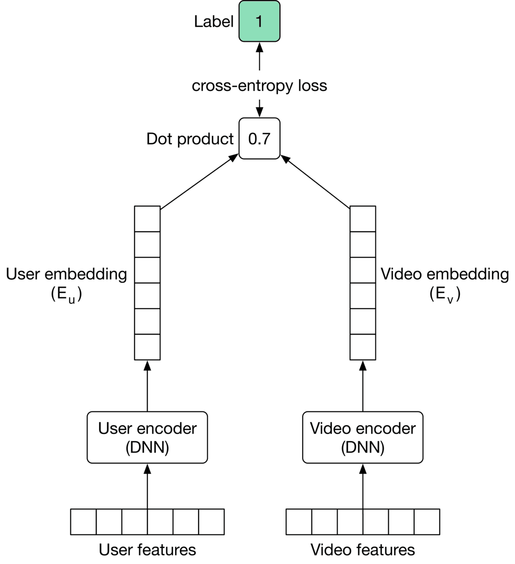
At inference time, the system uses the embeddings to find the most relevant videos for a given user. This is a classic "nearest neighbor" problem. We use approximate nearest neighbor methods to find the top most similar video embeddings efficiently.
Two-tower neural networks are used for both content-based filtering and collaborative filtering. When a two-tower architecture is used for collaborative filtering, as shown in Figure , the video encoder is nothing but an embedding layer that converts the video ID into an embedding vector. This way, the model doesn't rely on other video features.
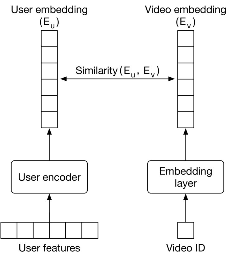
Let’s see the pros and cons of a two-tower neural network model.
Pros:
Cons:
Table 6.5 summarizes the differences between matrix factorization and two-tower neural network architecture.
| Matrix factorization | Two-tower neural network | |
|---|---|---|
| Training cost | ✓ More efficient to train | ✘ More costly to train |
| Inference speed | ✓ Faster as embeddings are static and can be precomputed | ✘ User features should be transformed into embeddings at query time |
| Cold-start problem | ✘ Cannot handle new users easily | ✓ Handles new users as it relies on user features |
| Quality of recommendations | ✘ Not ideal since the model does not use user/video features | ✓ Better recommendations since it relies on more features |
Table 6.5: Matrix factorization vs. two-tower neural networks
The system’s performance can be evaluated with offline and online metrics.
We evaluate the following offline metrics commonly used in recommendation systems.
Precision@k. This metric measures the proportion of relevant videos among the top recommended videos. Multiple values (e.g., ) can be used.
mAP. This metric measures the ranking quality of recommended videos. It is a good fit because the relevance scores are binary in our system.
Diversity. This metric measures how dissimilar recommended videos are to each other. This metric is important to track, as users are more interested in diversified videos. To measure diversity, we calculate the average pairwise similarity (e.g., cosine similarity or dot product) between videos in the list. A low average pairwise similarity score indicates the list is diverse.
Note that using diversity as the sole measure of quality can result in misleading interpretations. For example, if the recommended videos are diverse but irrelevant to the user, they may not find the recommendations helpful. Therefore, we should use diversity with other offline metrics to ensure both relevance and diversity.
In practice, companies track many metrics during online evaluation. Let's examine some of the most important ones:
CTR. The ratio between clicked videos and the total number of recommended videos. The formula is:
CTR is an insightful metric to track user engagement, but the drawback of CTR is that we cannot capture or measure clickbait videos.
The number of completed videos. The total number of recommended videos that users watch until the end. By tracking this metric, we can understand how often the system recommends videos that users watch.
Total watch time. The total time users spent watching the recommended videos. When recommendations interest users, they spend more time watching videos, overall.
Explicit user feedback. The total number of videos that users explicitly liked or disliked. The metric accurately reflects users' opinions of recommended videos.
At serving time, the system recommends the most relevant videos to a given user by narrowing the selection down from billions of videos. In this section, we will propose a prediction pipeline that's both efficient and accurate at serving requests.
Given we have billions of videos available, the serving speed would be slow if we choose a heavy model which takes lots of features as input. On the other hand, if we choose a lightweight model, it may not produce high-quality recommendations. So, what to do? A natural decision is to use more than one model in a multi-stage design. For example, in a two-stage design, a lightweight model quickly narrows down the videos during the first stage, called candidate generation. The second stage uses a heavier model that accurately scores and ranks the videos, called scoring. Figure shows how candidate generation and scoring work together to produce relevant videos.
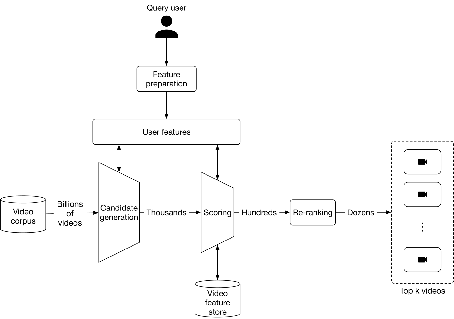
Let's take a closer look at the components of the prediction pipeline.
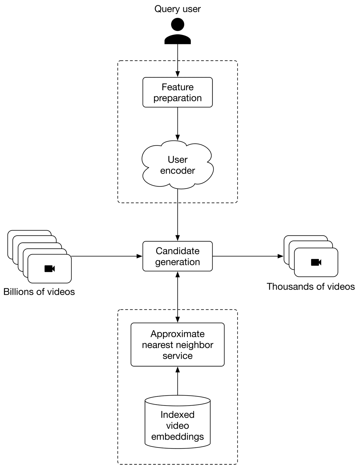
The goal of candidate generation is to narrow down the videos from potentially billions, to thousands. We prioritize efficiency over accuracy at this stage and are not concerned about false positives.
To keep candidate generation fast, we choose a model which doesn't rely on video features. In addition, this model should be able to handle new users. A two-tower neural network is a good fit for this stage.
Figure shows the candidate generation workflow. The candidate generation obtains a user's embedding from the user encoder. Once the computation is complete, it retrieves the most similar videos from the approximate nearest neighbor service. These videos are ranked based on similarity in the embedding space and are returned as the output.
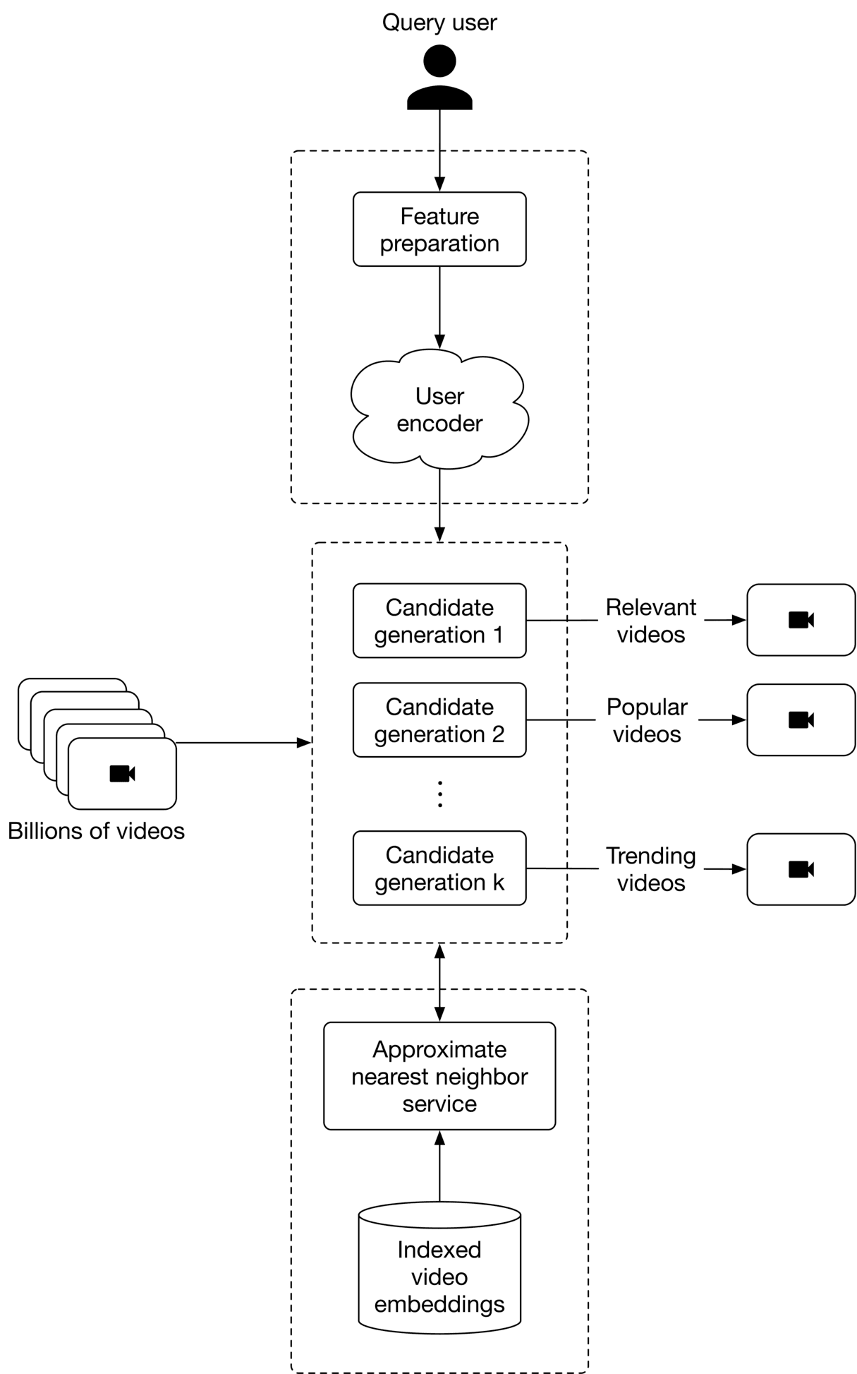
In practice, companies may choose to use more than one candidate generation because it could improve the performance of the recommendation. Let's take a look at why.
Users may be interested in videos for many reasons. For example, a user may choose to watch a video because it's popular, trending, or relevant to their location. To include those videos in the recommendations, it is common to use more than one candidate generation, as shown in Figure 6.25.
As soon as we have narrowed down potential videos from billions to thousands, we can use a scoring component to rank these videos before they are displayed.
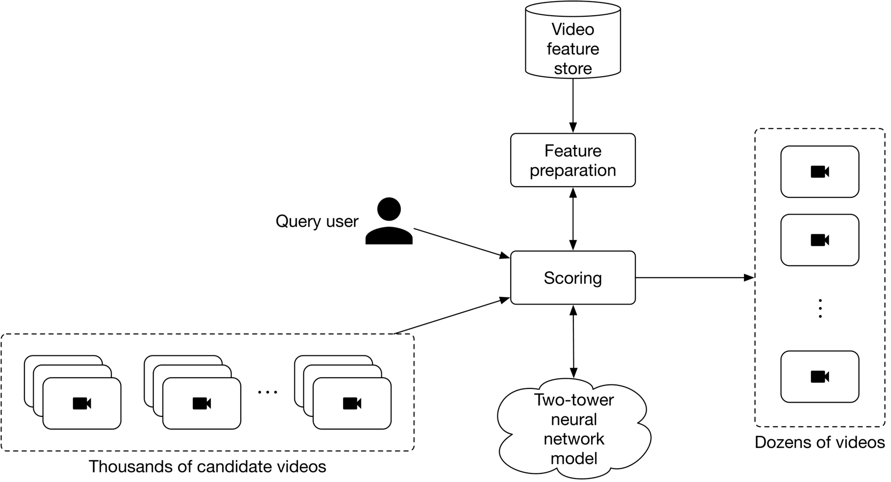
Also known as ranking, scoring takes the user and candidate videos as input, scores each video, and outputs a ranked list of videos.
At this stage, we prioritize accuracy over efficiency. To do so, we choose content-based filtering filtering and pick a model which relies on video features. A two-tower neural network is a common choice for this stage. Since there are only a handful of videos to rank in the scoring stage, we can employ a heavier model with more parameters. Figure 6.26 shows an overview of the scoring component.
This component re-ranks the videos by adding additional criteria or constraints. For example, we may use standalone ML models to determine if a video is clickbait. Here are a few important things to consider when building the re-ranking component:
Before wrapping up this chapter, let’s see how our design addresses typical challenges in video recommendation systems.
It is vital to recommend videos fast. However, as we have billions of videos in this system, recommending them efficiently and accurately is challenging. To address this issue, we used a two-stage design.
Specifically, we use a lightweight model in the first stage to quickly narrow down candidate videos from billions to thousands. YouTube uses a similar approach [2] , and Instagram adopts a multi-stage design [8].
To ensure precision, we employ a scoring component that ranks videos using a powerful model, which relies on more features, including video features. Using a more powerful model doesn't affect serving speed because only a small subset of videos is selected after the candidate generation phase.
Most users prefer to see a diverse selection of videos in their recommendations. To ensure our system produces a diverse set of videos, we adopt multiple candidate generators, as explained in the candidate generation section.
How does our system handle the cold-start problem?
For new users: We don't have any interaction data about new users when they begin using our platform.
In this case, predictions are made using two-tower neural networks based on features such as age, gender, language, location, etc. The recommended videos are personalized to some extent, even for new users. As the user interacts with more videos, we are able to make better predictions based on new interactions.
For new videos: When a new video is added to the system, the video metadata and content are available, but no interactions are present. One way to handle this is to use heuristics. We can display videos to random users and collect interaction data. Once we gather enough interactions, we fine-tune the two-tower neural network using the new interactions.
It's challenging to train models on large datasets in a cost-effective manner. In recommendation systems, new interactions are continuously added, and the models need to quickly adapt to make accurate recommendations. To quickly adapt to new data, the models should be able to be fine-tuned.
In our case, the models are based on neural networks and designed to be easily fine-tuned.
If there is time left at the end of the interview, here are some additional talking points: