
Design a data structure that supports adding integers from a data stream and retrieving the median of all elements received at any point.
add(num: int) -> None: adds an integer to the data structure.get_median() -> float: returns the median of all integers so far.Input: [add(3), add(6), get_median(), add(1), get_median()]
Output: [4.5, 3.0]
Explanation:
add(3)        # data structure contains [3] when sorted
add(6)        # data structure contains [3, 6] when sorted
get_median()  # median is (3 + 6) / 2 = 4.5
add(1)        # data structure contains [1, 3, 6] when sorted
get_median()  # median is 3.0
get_median is called.New to this one? Start here. Below is the core idea in everyday language, plus a real-world analogy—then the sections that follow build on it with the formal reasoning, code, and step-by-step walkthroughs.
Picture two buckets on a balance: a lower half (all the smaller numbers) and an upper half (all the bigger numbers). If you keep the buckets the same size, the median is sitting right at the pivot — it is the largest of the lower half, the smallest of the upper half, or the average of the two. Every new number gets dropped into the correct bucket, and we nudge the buckets back to balance.
The median is always found in the middle of a sorted list of values. The challenge with this problem is that it’s unclear how to keep all the values sorted as new values arrive, since the values don’t necessarily arrive in sorted order.
A useful point to recognize is that we don’t necessarily care if all the values are sorted. What really matters is that the median values are in their sorted positions. But is it possible to position these values in the middle without maintaining a fully sorted list of values? If it is, we’d need to find a way to differentiate the median values from the rest.
Consider the elements below, which contain an even number of values arranged in sorted order. The two values used to calculate the median are highlighted in the middle:
When a list contains two median values, we can make the following observations:
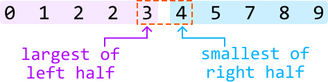
If we had a way to split the data into two halves, with one half containing the smaller values and the other half containing the larger values, we would just need an efficient method to identify the largest value in the smaller half, and the smallest value in the larger half. This is where heaps come in.
We can use a combination of a min-heap and a max-heap:
If the total number of elements is odd, there’s only one median. In this case, we just need to use one of the heaps to store it. Let's designate the max-heap to store this median:

Populating the heaps
Before identifying how we populate each heap, it’s useful to understand the behavior they must follow. Here are a couple of observations we can make:
All values in the left half must be less than or equal to any value in the right half.
The two halves should contain an equal number of values, except when the total number of values is odd, in which case the left half has one more value, as specified earlier.
These observations help us define two rules for managing the heaps:
The maximum value of the max-heap (left half) must be less than or equal to the minimum value of the min-heap (right half), ensuring all values in the left half are less than or equal to those in the right half.
The heaps should be of equal size, but the max-heap can have one more element than the min-heap.
Let's figure out how to maintain these rules in an example in which we try to add number 3 to the heaps. Note, the heaps before adding this number meet the above rules.
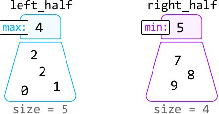
Since 3 is less than the maximum value of left_half (4), it belongs in the left_half heap. So, let’s add 3 to this heap:
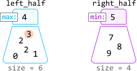
After adding 3, we notice rule 2 has been violated, since the size of the left_half heap is more than one element larger than the right_half heap. We can fix this by moving the max value of left_half to right_half:
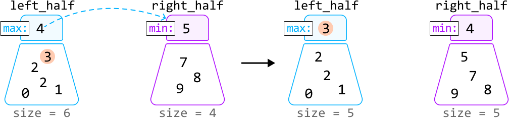
So, to ensure the sizes of the heaps don’t violate rule 2, we need to rebalance the heaps after adding a value:
left_half heap's size exceeds the right_half heap’s size by more than one, rebalance the heaps by transferring left_half‘s top value to right_half: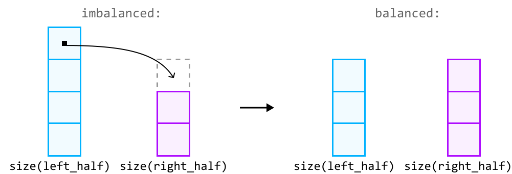
right_half heap’s size exceeds the left_half heap’s size, rebalance the heaps by transferring its top value to the left_half: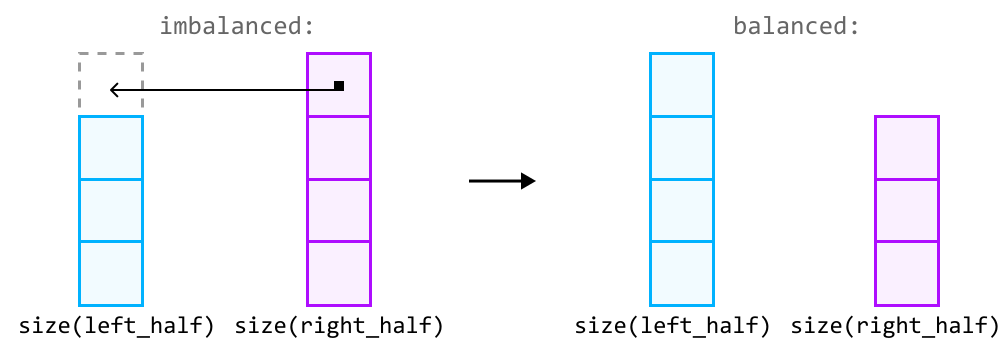
Returning the median
With the median values at the top of the heaps, returning the median boils down to two cases:
If the total number of elements is even, both median values can be found at the top of each heap. So, we return their sum divided by 2.
If the total number of elements is odd, the median will be at the top of the left_half heap.
Note that in Python, heaps are min-heaps by default. To mimic the functionality of a max-heap, we can insert numbers as negatives in the left_half heap. This way, the largest original value becomes the smallest when negated, positioning it at the top of the heap. When we retrieve a value from this heap, we multiply it by -1 to get its original value.
import heapq

class MedianOfAnIntegerStream:
    def __init__(self):
        # Max-heap for the values belonging to the left half.
        self.left_half = []
        # Min-heap for the values belonging to the right half.
        self.right_half = []

    def add(self, num: int) -> None:
        # If 'num' is less than or equal to the max of 'left_half', it belongs to the
        # left half.
        if not self.left_half or num <= -self.left_half[0]:
            heapq.heappush(self.left_half, -num)
            # Rebalance the heaps if the size of the 'left_half' exceeds the size of
            # the 'right_half' by more than one.
            if len(self.left_half) > len(self.right_half) + 1:
                heapq.heappush(self.right_half, -heapq.heappop(self.left_half))
        # Otherwise, it belongs to the right half.
        else:
            heapq.heappush(self.right_half, num)
            # Rebalance the heaps If 'right_half' is larger than 'left_half'.
            if len(self.left_half) < len(self.right_half):
                heapq.heappush(self.left_half, -heapq.heappop(self.right_half))

    def get_median(self) -> float:
        if len(self.left_half) == len(self.right_half):
            return (-self.left_half[0] + self.right_half[0]) / 2.0
        return -self.left_half[0]
struct MedianOfAnIntegerStream {
priority_queue<int> left; // max-heap (lower half)
priority_queue<int, vector<int>, greater<int>> right; // min-heap (upper half)
void add(int num) {
if (left.empty() || num <= left.top()) {
left.push(num);
if (left.size() > right.size() + 1) {
right.push(left.top()); // rebalance: left too big
left.pop();
}
} else {
right.push(num);
if (left.size() < right.size()) {
left.push(right.top()); // rebalance: right too big
right.pop();
}
}
}
double getMedian() {
if (left.size() == right.size()) {
return (left.top() + right.top()) / 2.0;
}
return left.top();
}
};class MedianOfAnIntegerStream {
private PriorityQueue<Integer> left = new PriorityQueue<>(Collections.reverseOrder()); // max-heap
private PriorityQueue<Integer> right = new PriorityQueue<>(); // min-heap
public void add(int num) {
if (left.isEmpty() || num <= left.peek()) {
left.offer(num);
if (left.size() > right.size() + 1) right.offer(left.poll());
} else {
right.offer(num);
if (left.size() < right.size()) left.offer(right.poll());
}
}
public double getMedian() {
if (left.size() == right.size()) return (left.peek() + right.peek()) / 2.0;
return left.peek();
}
}Time complexity:
add is , where denotes the number of values added to the data structure. This is because we first push a number to one of the heaps, which takes time. Then, if rebalancing is required, we also pop from one heap and push to the other, where both operations also take time.get_median is because accessing the top element of a heap takes time.Space complexity: The space complexity is because the two heaps together store elements.
Note: this explanation refers to the two middle values as "median values" to keep things simple. However, it’s important to understand that these two values aren’t technically “medians,” as there's only ever one median. These are just the two values used to calculate the median.
Two step-by-step walkthroughs of the algorithm below: a valid case (the expected happy path) and an invalid / edge case that exercises the tricky parts. Each step shows the program state as the code runs—the same steps apply to Python, C++ and Java.
top of a half (a median candidate) reported median
Left = lower half (max-heap, top on the right edge). Right = upper half (min-heap, top on the left edge).
| op | left (lower, max-heap) | right (upper, min-heap) | median |
|---|---|---|---|
| add 3 | [3] | [] | — |
| add 6 | [3] | [6] | — |
| median | [3] | [6] | (3+6)/2 = 4.5 |
| add 1 | [1,3] | [6] | — |
| median | [1,3] | [6] | top left = 3.0 |
top of a half moved across to rebalance reported median
Watch the value that hops across the pivot when a half grows too large.
| op | left (lower) | right (upper) | median |
|---|---|---|---|
| add 5,15 | [5] | [15] | — |
| add 1 | [1,5] | [15] | — |
| add 3 (rebal →) | [1,3] | [5,15] | — |
| median | [1,3] | [5,15] | (3+5)/2 = 4.0 |
| add 8 (rebal ←) | [1,3,5] | [8,15] | — |
| median | [1,3,5] | [8,15] | top left = 5.0 |
No real max-heap, so left_half stores -num. The largest lower value is -left_half[0]. Rebalancing moves a value by popping one heap and pushing (with a sign flip) into the other.
priority_queue<int> is a true max-heap for left; greater<int> makes right a min-heap. The logic reads exactly like the see-saw description — no sign tricks.
new PriorityQueue<>(Collections.reverseOrder()) gives the max-heap left; the default PriorityQueue is the min-heap right. peek reads a top, poll moves it across.