Determine if a target value exists in a matrix. Each row of the matrix is sorted in non-decreasing order, and the first value of each row is greater than or equal to the last value of the previous row.
Example:
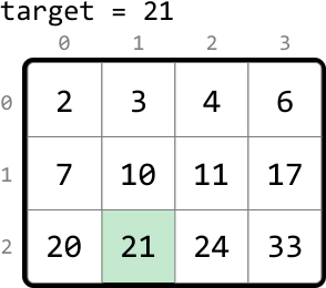
Output: True
Determine if a target value exists in a matrix. Each row of the matrix is sorted in non-decreasing order, and the first value of each row is greater than or equal to the last value of the previous row.
Output: True
New to this one? Start here. Below is the core idea in everyday language, plus a real-world analogy—then the sections that follow build on it with the formal reasoning, code, and step-by-step walkthroughs.
Read the grid the way you read a book: finish a line, drop to the start of the next line. Because every new row starts higher than the previous row ended, the numbers only ever increase as you read — it's really one long sorted list that happens to be written across several lines.
A naive solution to this problem is to linearly scan the matrix until we encounter the target value. However, this isn’t taking advantage of the sorted properties of the matrix.
A key observation is that all values in a given row are greater than or equal to all values in the previous row. This indicates the entire matrix can be considered as a single, continuous, sorted sequence of values:
![Image represents a data transformation process visualized using a matrix and arrows. A 3x4 matrix is shown, with rows labeled 0, 1, and 2, and columns labeled 0, 1, 2, and 3. Each cell in the matrix contains a numerical value (2, 3, 4, 6, 7, 10, 11, 17, 20, 21, 24, 33). Light orange arrows indicate data flow. Two arrows originate from the top-left corner of the matrix, one from row 0 and one from row 1, pointing downwards to a horizontal array below the matrix. This array displays the values from the first two rows of the matrix, concatenated horizontally ([2, 3, 4, 6, 7, 10, 11, 17]). A third arrow originates from the right side of the matrix, pointing downwards to another horizontal array, which displays the values from the last row of the matrix, concatenated horizontally ([20, 21, 24, 33]). The final output is a single horizontal array containing all the values from the matrix, arranged sequentially.](images/img-c454f71620e2.svg)
If we were able to flatten this matrix into a single, sorted array, we could perform a binary search on the array. Creating a separate array and populating it with the matrix’s values still takes time, and also takes space, where and are the dimensions of the matrix. Is there a way to perform a binary search on the matrix without flattening it?
Let’s map the indexes of the flattened array to their corresponding cells in the matrix:
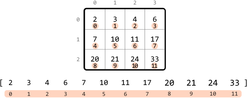
This index mapping would give us a way to access the elements of the matrix in a similar way to how we would access them in the flattened array. To figure out how to do this, let’s find a way to map any cell (r, c) to its corresponding index in the flattened array.
Let’s start by examining the mapped indexes of each row of the matrix:
n.n.From the above observations, we see a pattern: for any row r, the first cell of the row corresponds to the index r⋅n.
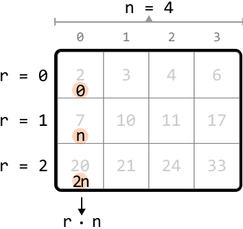
When we also consider the column value c, we can conclude that for any cell (r, c), the corresponding index in the flattened array is r⋅n + c.
Now that we understand how the 2D matrix maps to the 1D flattened array, let’s work backward to obtain the row and column indexes from an index in the flattened array. Let i = r⋅n + c. The row and column values are:
r = i // nc = i % nWe can see how these are obtained below:
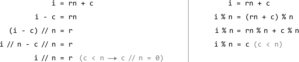
Now that we have these formulas, let’s use binary search to find the target.
Binary search
To define the search space, we need the first and last indexes of the flattened array. The first index is 0, and the last index is m⋅n - 1. So, we set the left and right pointers to 0 and m⋅n - 1 respectively.
To figure out how to narrow the search space, let’s explore an example matrix that contains the target of 21.
We can calculate mid using the formula: mid = (left + right) // 2. Then, determine the corresponding row and column values. Here, the value at the midpoint (10) is less than the target, which means the target is to the right of the midpoint. So, let’s narrow the search space toward the right:
![Image represents a visual explanation of a search algorithm within a 4x4 matrix. The top shows 'target = 21,' indicating the value being searched for. A 4x4 matrix is displayed below, with each cell containing a number and its row and column index shown as subscripts. The matrix is labeled with 'left', 'mid', and 'right' indicating index pointers. The 'mid' pointer highlights the value 10 at row 1, column 1. To the right, calculations are shown: 'r = mid // n' (integer division of 'mid' by 4, resulting in 1) and 'c = mid % n' (modulo operation of 'mid' by 4, resulting in 1). This determines the row (r=1) and column (c=1) of the element to check. The condition 'matrix[r][c] < target' (10 < 21) is shown, indicating that the element at row 1, column 1 is less than the target. Finally, the consequence 'left = mid + 1' is shown, suggesting the algorithm updates the 'left' pointer based on the comparison result. The highlighted cell (21) shows the target value found in the matrix.](images/img-8387a927711a.svg)
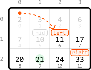
The new midpoint value is still less than the target, so let’s narrow the search space towards the right:
![Image represents a visual explanation of a search algorithm within a 4x4 matrix. The top shows 'target = 21,' indicating the value being searched for. A 4x4 matrix is displayed below, with rows labeled 0, 1, 2 and columns labeled 0, 1, 2, 3. Each cell contains a number, and the cell containing 20 is labeled 'mid' (in cyan), the cell containing 11 is labeled 'left' (in orange), and the cell containing 33 is labeled 'right' (in orange). To the right, a separate box details the calculation process: 'r = mid // n' (integer division of mid by n, where mid is 8 and n is 4, resulting in r=2) and 'c = mid % n' (modulo operation of mid by n, resulting in c=0). The line 'matrix[r][c] < target' indicates a comparison between the value at matrix position [2][0] (which is 20) and the target value (21). The result of this comparison (20 < 21) leads to the assignment 'left = mid + 1,' implying an adjustment of the search range based on the comparison. The overall diagram illustrates a step in a binary search or similar algorithm applied to a 2D array.](images/img-93ad508c2098.svg)
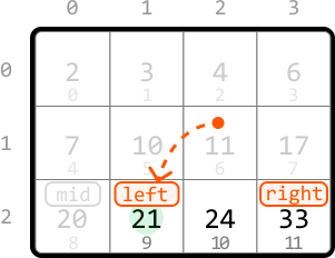
The midpoint value is now larger than the target, which means the target is to the left of the midpoint. So, let’s move the search space to the left:
![Image represents a visual explanation of a search algorithm within a 4x4 matrix. The top shows 'target = 21,' indicating the value being searched for. A 4x4 matrix is displayed below, with each cell containing a number and its row and column indices subtly indicated. The matrix's rows are indexed 0, 1, and 2, and columns are indexed 0, 1, 2, and 3. The number 21 is highlighted within the matrix, labeled 'left,' indicating its position in the search. To its right is the number 24, labeled 'mid,' and to its further right is 33, labeled 'right.' These labels suggest a binary search-like approach. A separate box to the right details the calculation process: 'r = mid // n' and 'c = mid % n' calculate the row (r) and column (c) indices of the 'mid' element (24 in this case), where 'mid' is 10 (its index in a flattened array), 'n' is 4 (the number of columns). The calculations show r = 2 and c = 2. Finally, 'matrix[r][c] > target → right = mid - 1' indicates that if the value at matrix[2][2] (which is 24) is greater than the target (21), the right boundary of the search is updated to 'mid - 1', effectively narrowing the search space.](images/img-e951f414b8c4.svg)
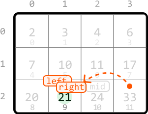
Now, the midpoint is equal to the target, so we return true to conclude the search.
![Image represents a visual explanation of a search algorithm within a matrix. A 3x4 matrix is shown, with each cell containing a number and its index (row, column) subtly displayed below. The top row displays column indices (0, 1, 2, 3), and the leftmost column displays row indices (0, 1, 2). The number 21 is highlighted within the matrix at index (2,1), indicating a 'mid' value. To the right, a separate box details the calculation: `r = mid // n` (integer division of `mid` (9) by `n` (4), resulting in `r = 2`) and `c = mid % n` (modulo operation of `mid` (9) by `n` (4), resulting in `c = 1`). This calculation determines the row (`r`) and column (`c`) indices of the element being checked. Finally, the condition `matrix[r][c] == target` is shown, indicating that if the element at the calculated index (`matrix[2][1]`) equals the `target` value (21), the function returns `True`. The overall diagram illustrates how a search algorithm might locate a target value within a matrix using integer division and modulo operations to determine the index.](images/img-5deddfdbeb6f.svg)
Note that our exit condition should be while left ≤ right in order to also examine the above search space when left == right.
from typing import List

def matrix_search(matrix: List[List[int]], target: int) -> bool:
    m, n = len(matrix), len(matrix[0])
    left, right = 0, m * n - 1
    # Perform binary search to find the target.
    while left <= right:
        mid = (left + right) // 2
        r, c = mid // n, mid % n
        if matrix[r][c] == target:
            return True
        elif matrix[r][c] > target:
            right = mid - 1
        else:
            left = mid + 1
    return False
bool matrixSearch(vector<vector<int>>& matrix, int target) {
if (matrix.empty() || matrix[0].empty()) {
return false;
}
int m = (int)matrix.size(), n = (int)matrix[0].size();
int left = 0, right = m * n - 1;
while (left <= right) {
int mid = left + (right - left) / 2;
int value = matrix[mid / n][mid % n]; // flat index -> (row, col)
if (value == target) {
return true;
} else if (value < target) {
left = mid + 1;
} else {
right = mid - 1;
}
}
return false;
}public boolean matrixSearch(int[][] matrix, int target) {
if (matrix.length == 0 || matrix[0].length == 0) return false;
int m = matrix.length, n = matrix[0].length;
int left = 0, right = m * n - 1;
while (left <= right) {
int mid = left + (right - left) / 2;
int value = matrix[mid / n][mid % n]; // flat index -> (row, col)
if (value == target) return true;
else if (value < target) left = mid + 1;
else right = mid - 1;
}
return false;
}Time complexity: The time complexity of matrix_search is because it performs a binary search over a search space of size .
Space complexity: The space complexity is .
Two step-by-step walkthroughs of the algorithm below: a valid case (the expected happy path) and an invalid / edge case that exercises the tricky parts. Each step shows the program state as the code runs—the same steps apply to Python, C++ and Java.
left mid right found thrown away
left = 6.
right = 7.
left = 7.
| left | right | mid | (row, col) | value | action |
|---|---|---|---|---|---|
| 0 | 11 | 5 | (1, 1) | 11 | 11 < 20 → left = 6 |
| 6 | 11 | 8 | (2, 0) | 23 | 23 > 20 → right = 7 |
| 6 | 7 | 6 | (1, 2) | 16 | 16 < 20 → left = 7 |
| 7 | 7 | 7 | (1, 3) | 20 | match → return true |
left mid right thrown away
left = 6.
left = 9.
left = 11.
right = 10. Now left (11) > right (10).
left = 11 > right = 10 → the window is empty. 45 was never found → return false.
| left | right | mid | (row, col) | value | action |
|---|---|---|---|---|---|
| 0 | 11 | 5 | (1, 1) | 11 | 11 < 45 → left = 6 |
| 6 | 11 | 8 | (2, 0) | 23 | 23 < 45 → left = 9 |
| 9 | 11 | 10 | (2, 2) | 34 | 34 < 45 → left = 11 |
| 11 | 11 | 11 | (2, 3) | 60 | 60 > 45 → right = 10 |
| 11 | 10 | — | — | — | window empty → return false |
The flat-index steps match the tables above. Python-specific: value = matrix[mid // n][mid % n] (floor division), guarded by if not matrix or not matrix[0].
Same steps. C++-specific: matrix[mid / n][mid % n], guarded by matrix.empty() || matrix[0].empty().
Same steps. Java-specific: matrix[mid / n][mid % n], guarded by matrix.length == 0 || matrix[0].length == 0.