Return the node where two singly linked lists intersect. If the linked lists don't intersect, return null.

Example:
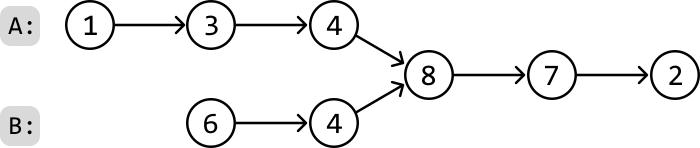
The image represents a directed acyclic graph (DAG) illustrating two distinct paths, labeled 'A:' and 'B:'.  Path 'A:' starts with a node labeled '1', which connects to a node labeled '3', followed by a node labeled '4'. Node '4' then branches, connecting to a node labeled '8'. Path 'B:' begins with a node labeled '6', connecting to another node labeled '4'. This second '4' node also connects to node '8'. Node '8' subsequently connects to a node labeled '7', which finally connects to a node labeled '2'.  The arrows indicate the direction of flow between the nodes, showing a sequential progression along each path.  The paths 'A' and 'B' represent different sequences or processes, converging at node '8' before diverging again.  The numbers within the nodes likely represent steps or stages in a process, and the overall structure suggests a workflow or dependency diagram.
Output: Node 8

In Plain English

New to this one? Start here. Below is the core idea in everyday language, plus a real-world analogy—then the sections that follow build on it with the formal reasoning, code, and step-by-step walkthroughs.

🌱 Real-world analogy: two roads that merge onto one highway

Two on-ramps of different lengths feed into the same highway. If two cars leave the start of each ramp at the same speed, the one on the shorter ramp reaches the merge first and pulls ahead. To make them arrive together, give each car a clever route: drive your ramp, then drive the other car's ramp. Now both cars travel the exact same total distance, so they reach the merge point at the same instant.

Intuition

Let’s first understand what an intersection between two linked lists is.

An intersection occurs when two linked lists converge at a shared node and, from that point onwards, share all subsequent nodes.

Note, this intersection has nothing to do with the values of the nodes.

A naive approach is to use a hash set. We can traverse the first linked list once and store each node in a hash set. Next, we traverse the second linked list until we find the first node that exists in the hash set, signifying the intersection point since it’s the first node shared between the two linked lists. This approach solves the problem linearly, but can we find a solution that uses constant space?

Consider the following example:
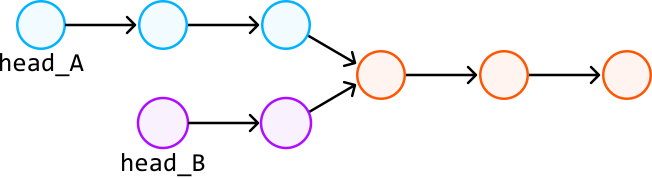
Image represents a diagram illustrating a merge operation in a linked list data structure.  Two linked lists, labeled 'head_A' and 'head_B,' are depicted.  List 'head_A' consists of three light-blue nodes connected sequentially by unidirectional arrows, indicating the flow of data. Similarly, list 'head_B' comprises two light-purple nodes linked in the same manner.  The final nodes of both lists 'head_A' and 'head_B' converge at a common node, the first of a new linked list represented by three orange nodes. These orange nodes are also connected sequentially with unidirectional arrows. The arrows visually represent the pointers connecting the nodes in each list, showing the direction of traversal. The overall structure demonstrates how two separate linked lists are merged into a single, unified list.

Treating these as two separate linked lists can get confusing with the above visualization. Instead, let’s visualize the input as two linked lists to help us think about the problem more clearly. Note that the tail nodes are still shared between the two linked lists, we’re just visualizing them separately:
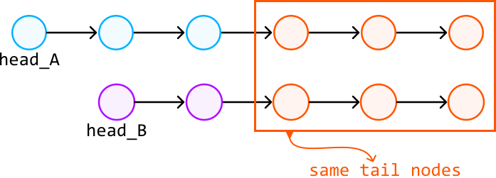
The image represents two linked lists merging into a single structure.  Two lists, labeled `head_A` and `head_B`, are depicted using light-blue and light-purple circles respectively, representing nodes, connected by black arrows indicating the direction of traversal.  Each list consists of three nodes.  These lists converge at a point where they share a common set of nodes, represented by three peach-colored circles enclosed within an orange rectangle.  These shared nodes are labeled as 'same tail nodes' via a curved arrow pointing to the rectangle. The arrangement visually demonstrates how two separate linked lists can share a common tail section, a concept relevant to data structure optimization and merging algorithms.

Notice that this problem is easier to solve if the two linked lists are of equal length. This is because the intersection node can be found at the same position from the heads of both linked lists. In other words, when we iterate through two linked lists of the same length, we’re guaranteed to reach the intersection node at the same time:
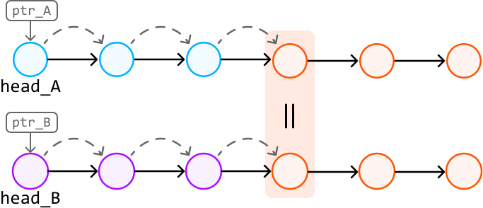
Image represents two linked lists, labeled 'A' and 'B', visually separated by a peach-colored rectangle containing the symbol '||' signifying a parallel structure.  List 'A' uses light-blue nodes, while list 'B' uses light-purple nodes. Each list starts with a labeled head node ('head_A' and 'head_B'), pointed to by a rectangular box labeled 'ptr_A' and 'ptr_B' respectively, indicating pointers to the beginning of each list.  Solid arrows show the sequential connections within each list. Dashed gray arrows indicate additional pointers, possibly for iterative traversal or other operations, connecting nodes within each list.  Both lists converge at a point represented by orange nodes, forming a common section after the initial distinct parts.  The orange nodes continue in a linked list structure, suggesting a merging or concatenation of the two initial lists.

Could we somehow replicate this behavior when dealing with linked lists of varying lengths? The key observation is that, while two linked lists ‘list A’ and ‘list B’ may have different lengths, ‘list A → list B’ has the same length as ‘list B → list A’ (where ‘→’ represents the connection of two lists). Conveniently, these combined linked lists also share the same tail nodes:
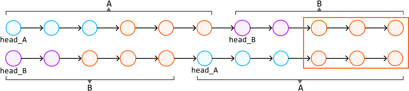
Image represents two linked lists, A and B, initially separate, depicted as horizontal sequences of circles connected by arrows indicating direction.  List A starts with a light-blue circle labeled 'head_A' and continues with several light-blue and orange circles. List B begins with a light-purple circle labeled 'head_B' and proceeds with light-purple and orange circles.  The lists merge; the tail of list A connects to a light-blue circle, which is then followed by several more light-blue circles, and the tail of list B connects to a light-purple circle, followed by several more light-purple circles.  After the merge, a rectangular box encloses a section of the combined lists, containing four orange circles arranged in two rows of two, representing a sub-section of the merged list.  The labels 'A' and 'B' are placed above and below the initial sections of lists A and B respectively, indicating their initial separation, and are reversed below the merged section, indicating the merging point.  Arrows consistently point rightward, showing the direction of traversal through each list.

We’ve now set up a scenario where we have two combined linked lists of the same length, which share the same tail nodes. By traversing these combined linked lists, we’ll eventually reach the intersection node simultaneously on both linked lists (if one exists).

To do this, we can traverse both combined linked lists with two pointers, and stop once the nodes at both pointers are the same. This node would be the intersection node:
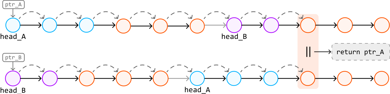
Image represents two linked lists, A and B, visualized horizontally.  List A's nodes are light blue, while list B's nodes are light purple.  Both lists also contain orange nodes interspersed.  A rectangular box labeled 'ptr_A' points down to the head of list A, labeled 'head_A,' which is a light blue circle.  Similarly, a box labeled 'ptr_B' points to the head of list B, 'head_B,' a light purple circle.  Solid arrows indicate the forward links within each list. Dashed gray arrows show how the algorithm iterates through both lists simultaneously, comparing nodes.  The lists merge at a point where list A's orange node connects to list B's purple node, and vice-versa.  After the merging point, the lists continue with their respective node colors. A peach-colored rectangle separates the merged portion from the rest of the lists. A solid arrow emerges from this rectangle, pointing to a dashed-line box labeled 'return ptr_A,' indicating that the algorithm returns a pointer to a node within list A after the merging process.

If no intersection exists, both pointers will end up stopping at null nodes:
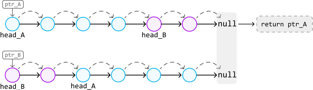
Image represents two linked lists, A and B, visualized horizontally.  List A's head is labeled 'head_A' and is a light-blue circle; list B's head is labeled 'head_B' and is a purple circle.  Each list consists of several nodes represented by similarly colored circles connected by solid arrows indicating the next node in the sequence.  Above each list's head is a rectangular box labeled 'ptr_A' and 'ptr_B' respectively, representing pointers to the respective list heads.  Dashed arrows from these pointer boxes point to the respective list heads, showing the pointer's initial position.  Both lists terminate with a 'null' node represented by a light-grey rectangle.  After the 'null' nodes, a solid arrow points to a dashed-line rectangle labeled 'return ptr_A', indicating that the function returns a pointer to the head of list A.  The dashed arrows between the nodes in each list suggest the traversal of the list during the execution of the algorithm.  The arrangement shows the lists' structure and the pointer's role in accessing and manipulating the lists.

Traversing combined linked lists
An important observation is that to traverse through 'list A → list B', we don't actually need to connect these two linked lists together. Instead, we can traverse 'list A' and, upon reaching its end, continue by traversing 'list B':
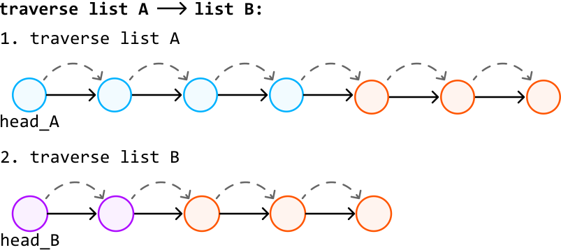
Image represents a diagram illustrating the traversal of two linked lists, A and B.  The top section, labeled '1. traverse list A,' shows a linked list A depicted as a sequence of four light-blue circles connected by solid black arrows, representing the nodes and their connections.  The first node is labeled 'head_A'.  Dashed grey arrows curve above the solid arrows, indicating the traversal process. The bottom section, labeled '2. traverse list B,' similarly shows a linked list B with three light-purple circles followed by three peach-colored circles, connected by solid black arrows. The first node is labeled 'head_B,' and dashed grey arrows above the solid arrows again show the traversal.  The title 'traverse list A → list B:' indicates that the diagram demonstrates a process involving traversing both lists, possibly for comparison or data transfer between them.  The color change in list B suggests a potential modification or interaction during the traversal.

This technique allows us to traverse the entire sequence of both linked lists as if they were connected.

Implementation

from ds import ListNode
   
def linked_list_intersection(head_A: ListNode, head_B: ListNode) -> ListNode:
    ptr_A, ptr_B = head_A, head_B
    # Traverse through list A with 'ptr_A' and list B with 'ptr_B' until they meet.
    while ptr_A != ptr_B:
        # Traverse list A -> list B by first traversing 'ptr_A' and then, upon
        # reaching the end of list A, continue the traversal from the head of list B.
        ptr_A = ptr_A.next if ptr_A else head_B
        # Simultaneously, traverse list B -> list A.
        ptr_B = ptr_B.next if ptr_B else head_A
    # At this point, 'ptr_A' and 'ptr_B' either point to the intersection node or both
    # are null if the lists do not intersect. Return either pointer.
    return ptr_A
ListNode* linkedListIntersection(ListNode* headA, ListNode* headB) {
    ListNode* a = headA;
    ListNode* b = headB;
    while (a != b) {                       // compare pointers, not values
        a = (a != nullptr) ? a->next : headB;  // ran off A? jump to B
        b = (b != nullptr) ? b->next : headA;  // ran off B? jump to A
    }
    return a;                              // the shared node, or nullptr
}
public ListNode linkedListIntersection(ListNode headA, ListNode headB) {
    ListNode a = headA;
    ListNode b = headB;
    while (a != b) {                       // compare references, not values
        a = (a != null) ? a.next : headB;  // ran off A? jump to B
        b = (b != null) ? b.next : headA;  // ran off B? jump to A
    }
    return a;                              // the shared node, or null
}

Complexity Analysis

Time complexity: The time complexity of linked_list_intersection is O(n+m)O(n+m), where nn and mm denote the lengths of list A and B, respectively. This is because pointers linearly traverse both linked lists sequentially.

Space complexity: The space complexity is O(1)O(1).

Dry Runs

Two step-by-step walkthroughs of the algorithm below: a valid case (the expected happy path) and an invalid / edge case that exercises the tricky parts. Each step shows the program state as the code runs—the same steps apply to Python, C++ and Java.

✅ Dry run 1 (valid) — A = 2→3→7→8, B = 5→7→8 share the tail 7→8 (lenA = 4, lenB = 3).

pointer a pointer b shared tail

The lists. Both end in the same 7 → 8 (identical nodes). We want to return that 7.
A
2
3
7
8
null
B
5
7
8
null
The switch. a reaches the end of A first (shorter walk) and jumps to head B; b later jumps to head A. From then on they are aligned.
a walks
2
3
7
8
5
7
8?
b walks
5
7
8
2
3
7?
They meet. After equal total distance, a and b land on the same node 7 → return it. 🎉
2
3
7ab
8
null

The same run as a table

Node each pointer sits on. = null (then it jumps to the other head). Meeting is by identity.
itera onb ona == b?
02 (A)5 (B)no
13 (A)7 (shared)no
27 (shared)8 (shared)no
38 (shared)∅ → jumpno
4∅ → jump2 (A)no
55 (B)3 (A)no
67 (shared)7 (shared)yes → return 7
📈 Dry run 2 (invalid) — A = 2→3→7, B = 9→5 are disjoint → return null.

pointer a pointer b

The lists (disjoint). A and B share no node, so the correct answer must be null.
A
2
3
7
null
B
9
5
null
Each pointer walks both lists. a: 2→3→7→→(jump to B)→9→5. b: 9→5→→(jump to A)→2→3→7. Each covers lenA + lenB = 5 nodes.
a walks
2
3
7
9
5
b walks
9
5
2
3
7
They meet at null. After equal total distance both pointers step off the end at the same moment: a == b == null. The loop ends and we return null. ✅
nullab

The same run as a table

Node each pointer sits on. = null (then it jumps to the other head). With no join, the only meeting point is null.
itera onb ona == b?
02 (A)9 (B)no
13 (A)5 (B)no
27 (A)∅ → jump to Ano
3∅ → jump to B2 (A)no
49 (B)3 (A)no
55 (B)7 (A)no
6yes → both null → return null

Contrast with Dry run 1: there the pointers coincided on a real node (the join). Here there is no join, so the only place they can coincide is null — and because each walks exactly lenA + lenB nodes, they arrive there together. That is why the switch uses the other head at null instead of skipping null.

The same steps in each language

Both runs step exactly as the tables above. Python compares identity with a is not b; on reaching the end it switches with a = a.next if a else headB.

Same steps. C++ compares the pointers with a != b; the switch is a = a ? a->next : headB;

Same steps. Java compares the references with a != b; the switch is a = (a != null) ? a.next : headB;