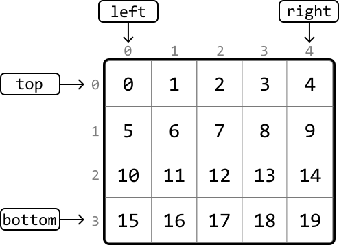
Return the elements of a matrix in clockwise spiral order.

Example:
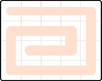
Image represents a grid-based diagram illustrating a linear data structure traversal pattern, possibly demonstrating a specific algorithm or data flow.  The diagram shows a sequence of numbered nodes (0-19) arranged in a snake-like path across a 5x4 grid.  Each node is represented by a number within a peach-colored rectangle.  Orange arrows connect adjacent nodes, indicating the direction of traversal. The path starts at node 0, proceeds rightward to node 4, then downwards, traversing nodes 9, 14, and 19.  From node 4, the path turns downwards to node 9, then downwards again to node 14, and finally to node 19.  The path then reverses direction at node 19, moving leftward to node 18, and continues leftward and upward, forming a loop that eventually connects back to node 5, then to node 10, and finally to node 15.  The overall structure resembles a snake winding through the grid, demonstrating a non-standard linear traversal order.
Output: [0, 1, 2, 3, 4, 9, 14, 19, 18, 17, 16, 15, 10, 5, 6, 7, 8, 13, 12, 11]

In Plain English

New to this one? Start here. Below is the core idea in everyday language, plus a real-world analogy—then the sections that follow build on it with the formal reasoning, code, and step-by-step walkthroughs.

🧍 Real-world analogy: peeling an onion layer by layer

Reading a grid in a spiral is like peeling an onion: strip off the whole outer layer (top row, right column, bottom row, left column), then peel the next layer inward, and so on until nothing is left. Four shrinking boundaries — top, bottom, left, right — track which layer you are on.

One Big Idea

Track four boundaries — top, bottom, left, right. Walk one edge, then pull that boundary inward so it is never revisited. Repeat while the boundaries have not crossed. No visited grid needed — O(1) extra space.

Intuition

To create the expected output for this problem, let's try simulating exactly what the problem describes and traverse the matrix in spiral order, adding each value to the output as we go. How can we do this?

Spiral traversal involves moving through the matrix in one direction until we can't go any further, then changing direction and continuing. Specifically, the sequence of directions is right, down, left, and up, repeated until all elements are traversed. To achieve this, we need to determine the exact conditions for switching directions.

Initially, our approach may seem simple: we start by moving right until reaching the right-most column of the matrix, at which point we switch directions. We can move and switch directions like this three times without running into any problems:
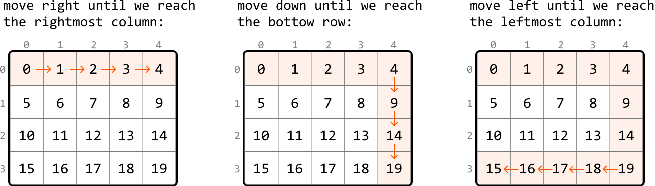
Image represents three 4x4 matrices illustrating different traversal patterns. Each matrix contains numbers from 0 to 19 arranged sequentially.  The first matrix shows a rightward traversal, indicated by orange right-pointing arrows connecting the numbers 0 through 4 in the first row, then continuing to the next row and so on. Above this matrix, text reads 'move right until we reach the rightmost column:'. The second matrix demonstrates a downward traversal, with orange downward-pointing arrows connecting the numbers 4, 9, 14, and 19, positioned in the last column.  The text above it reads 'move down until we reach the bottom row:'. The third matrix depicts a leftward traversal, using orange left-pointing arrows connecting the numbers 19, 18, 17, and 15 in the last row, then continuing to the previous row and so on.  The text above this matrix reads 'move left until we reach the leftmost column:'.  All three matrices share the same numerical arrangement, but the arrows highlight different paths through the data.  Row and column indices (0-3) are displayed along the top and left side of each matrix.

However, as shown below, if we move upward until we hit the top row of the matrix, we'll return to where we started, adding a value from a previously visited cell to the output:
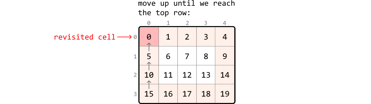
Image represents a 4x5 grid illustrating a coding pattern.  The grid is labeled with row numbers (0, 1, 2, 3) on the left and column numbers (0, 1, 2, 3, 4) at the top. Each cell contains a number from 0 to 19, sequentially arranged.  The top-left cell (0,0) is highlighted in light red and labeled as the 'revisited cell'.  A red arrow points from the text 'revisited cell' to this cell (0,0).  Within the grid, upward-pointing grey arrows are shown originating from cells (1,0), (2,0), and (3,0), indicating a movement upwards towards the top row. The text above the grid, 'move up until we reach the top row:', describes the process depicted by the arrows, suggesting an upward traversal of the grid from a specific cell until the top row is reached.

A potential solution to this is to keep track of all cells visited by using a hash set. This allows us to stop moving in a direction when we encounter a visited cell. While this approach is effective, it requires O(mn)O(m\cdot n) space, where mm and nn are the dimensions of the matrix. This is because we need to store every cell of the matrix in the hash set. Is there a way to avoid revisiting cells without using an additional data structure?

Notice in the above diagrams that when we move in a certain direction, we continue until we reach one of the boundary rows or columns (i.e., the top or bottom row, or the leftmost or rightmost column).

What if we adjust these boundaries as we traverse the matrix, to avoid revisiting previous cells?

Adjusting boundaries
Let's initialize the four boundaries (top, bottom, left, right) with their initial positions:

Image represents a 4x5 matrix of numbers from 0 to 19, visually illustrating a 2-dimensional array.  The matrix is labeled with numbers 0-4 across the top and 0-3 down the left side, representing row and column indices respectively.  The numbers within the matrix are arranged sequentially, increasing from left to right and top to bottom.  Four rectangular boxes labeled 'left,' 'right,' 'top,' and 'bottom' are positioned outside the matrix. Arrows indicate data flow: 'left' points down to the top-left corner (0,0) of the matrix, 'right' points down to the top-right corner (0,4), 'top' points right to the leftmost column (0), and 'bottom' points right to the bottom-most column (3). This arrangement suggests a visual representation of how data might be accessed or traversed within a 2D array using different starting points or directions.

We begin traversal by moving right through the first row from the left boundary to the right. Since we've just visited all cells in the first row, we need to prevent future access to this row. This can be done by moving the top boundary down by 1 (top += 1), ensuring the top row can't be accessed:
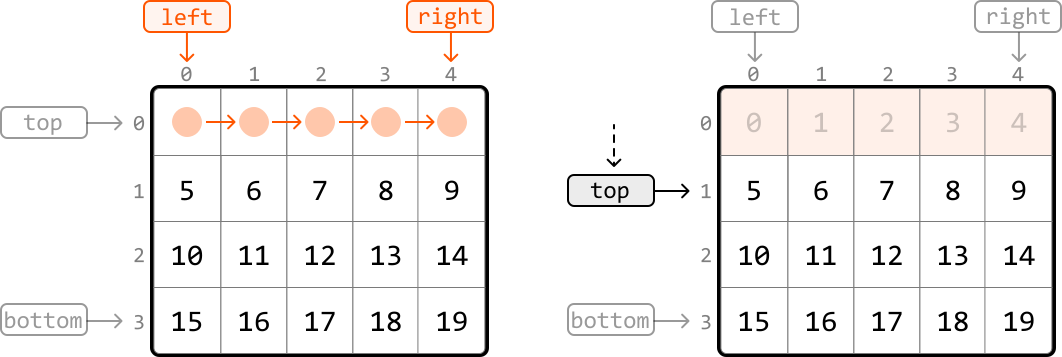
Image represents a comparison of two data structures, both 4x4 matrices.  The left matrix visually demonstrates data traversal.  It contains numbers 0-19 arranged in a grid, with the top row (0-4) highlighted in peach circles and connected by rightward arrows, indicating a sequential traversal from left to right.  Labels 'left' and 'right' (orange boxes) point to the starting and ending points of this traversal, respectively.  Labels 'top' and 'bottom' (grey boxes) indicate the entry and exit points for the data flow into and out of the matrix. The right matrix shows the same numerical data but without the highlighted traversal.  A dotted arrow connects the 'top' label of the left matrix to the 'top' label of the right matrix, suggesting a transformation or mapping between the two structures.  The right matrix's top row (0-4) is shaded light beige, possibly indicating a different state or highlighting a specific aspect of the data.  Both matrices are labeled with row and column indices (0-3 and 0-4 respectively), providing a clear coordinate system for data access.

Next, we move down from the top boundary to the bottom boundary. To ensure this column is not revisited, update the right boundary (right -= 1):
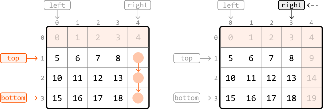
Image represents a comparison of two 5x5 matrices before and after a rightward shift operation.  The left matrix shows a 5x5 grid with numbers from 0 to 24 arranged sequentially, row by row.  Orange rectangular boxes labeled 'top' and 'bottom' indicate data input from the top and bottom, respectively.  Grey rectangular boxes labeled 'left' and 'right' indicate the column indices.  Within the matrix, the numbers 9, 14, and 19 are highlighted in peach circles.  An orange arrow points from the 'top' box to the first row of the matrix, and another from the 'bottom' box to the third row.  A downward orange arrow connects the highlighted numbers 9, 14, and 19, indicating a vertical flow of data. The right matrix depicts the result after a rightward shift. The numbers 9, 14, and 19 have moved to the rightmost column, with the rightmost column's original values (9, 14, 19) now appearing as light peach-colored numbers. A grey arrow points from the 'top' box to the first row of the right matrix, and another from the 'bottom' box to the third row. A dashed grey arrow points from the right matrix to the 'right' label, indicating the output of the shift operation.  The 'left' label remains unchanged, indicating that the leftmost column remains unaffected.

Next, we move left from the right boundary to the left. To ensure this row doesn't get revisited, update the bottom boundary (bottom -= 1):
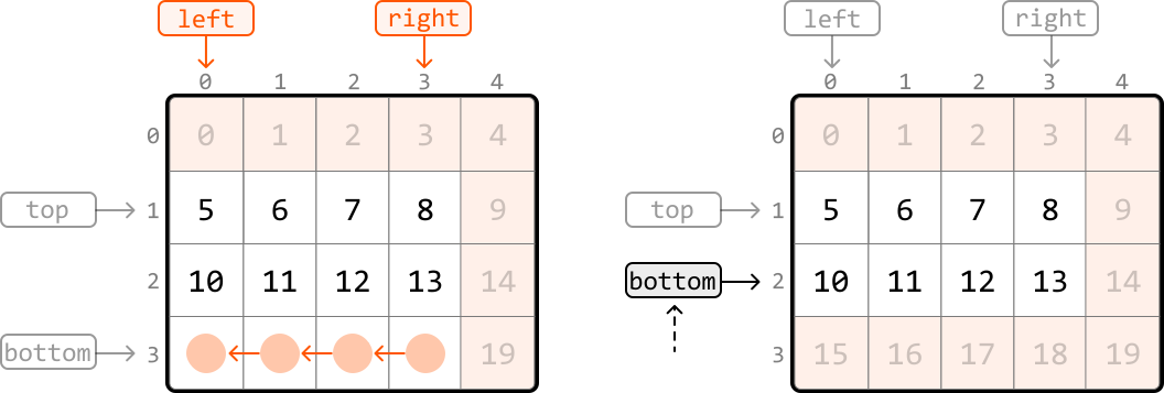
Image represents two 5x5 matrices, each labeled with row and column indices from 0 to 4.  The first matrix contains numbers 0-19 arranged sequentially, row by row.  The second matrix is initially identical.  Above each matrix are orange rectangular boxes labeled 'left' and 'right,' indicating directional input.  To the left of both matrices are gray rectangular boxes labeled 'top' and 'bottom,' representing input sources.  Arrows show data flow: 'top' feeds into row 1 of both matrices, 'bottom' feeds into row 3 of both matrices, 'left' feeds into column 0, and 'right' feeds into column 3.  In the first matrix, the numbers 15, 16, 17, and 18 in the bottom row are highlighted in peach.  In the second matrix, these same numbers are highlighted and connected by bidirectional arrows, illustrating a data transformation or interaction specifically within the bottom row, possibly representing a data flow or manipulation within a specific section of the matrix.

Next, we move up from the bottom boundary to the top boundary. To ensure this column isn't revisited, update the left boundary (left += 1):
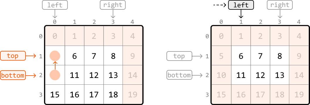
Image represents a visual depiction of data transformation or flow within a coding pattern, possibly related to matrix manipulation or data indexing.  The image is divided into two main sections, each showing a 4x5 matrix with numerical values (0-19) arranged sequentially.  The left section displays the initial matrix, with values 5 and 10 highlighted in peach circles at coordinates (1,0) and (2,0) respectively.  Above this matrix, labels 'left' and 'right' indicate column headers, and numbers 0-4 represent row indices.  Orange rectangular boxes labeled 'top' and 'bottom' show data input sources, with arrows indicating data flow into the matrix at row indices 1 and 2 respectively, targeting the highlighted cells. The right section shows the transformed matrix after the data flow.  The 'top' input (from the left section) is shown flowing into row 1, and the 'bottom' input flows into row 2.  A dashed arrow points from the 'left' label in the left section to the 'left' label in the right section, suggesting a potential data transformation or mapping process affecting the column headers.  The numbers in the right matrix are identical to the left except for the highlighted cells, which remain unchanged, illustrating a selective update operation.

We've just discussed how to traverse in each of the four directions and update the corresponding boundaries. These traversals are repeated until either the top boundary surpasses the bottom boundary, or the left boundary surpasses the right boundary. Either of these indicate there are no more cells left to traverse.


In summary, we traverse the matrix in spiral order by repeating the following sequences of traversals:

  1. Move from left to right along the top boundary, then update the top boundary (top += 1)

  2. Move from top to bottom along the right boundary, then update the right boundary (right -= 1)

  3. Move from right to left along the bottom boundary, then update the bottom boundary (bottom -= 1)

  4. Move from bottom to top along the left boundary, then update the left boundary (left += 1)

This continues while top ≤ bottom and left ≤ right.

A crucial thing to keep in mind is that after updating the top boundary, the top boundary might pass the bottom boundary (top > bottom). So, we need to check that top ≤ bottom before traversing the bottom boundary. Similarly, we need to check that left ≤ right before traversing the left boundary to ensure the boundaries haven't crossed.

As we move through the matrix, we add each value we encounter to the output array. This way, the matrix values are recorded in a spiral order.

Implementation

from typing import List
    
def spiral_matrix(matrix: List[List[int]]) -> List[int]:
    if not matrix:
        return []
    result = []
    # Initialize the matrix boundaries.
    top, bottom = 0, len(matrix) - 1
    left, right = 0, len(matrix[0]) - 1
    # Traverse the matrix in spiral order.
    while top <= bottom and left <= right:
        # Move from left to right along the top boundary.
        for i in range(left, right + 1):
            result.append(matrix[top][i])
        top += 1
        # Move from top to bottom along the right boundary.
        for i in range(top, bottom + 1):
            result.append(matrix[i][right])
        right -= 1
        # Check that the bottom boundary hasn't passed the top boundary before
        # moving from right to left along the bottom boundary.
        if top <= bottom:
            for i in range(right, left - 1, -1):
                result.append(matrix[bottom][i])
            bottom -= 1
        # Check that the left boundary hasn't passed the right boundary before
        # moving from bottom to top along the left boundary.
        if left <= right:
            for i in range(bottom, top - 1, -1):
                result.append(matrix[i][left])
            left += 1
    return result
vector<int> spiralMatrix(vector<vector<int>>& matrix) {
    vector<int> result;
    if (matrix.empty() || matrix[0].empty()) {
        return result;
    }
    int top = 0, bottom = (int)matrix.size() - 1;
    int left = 0, right = (int)matrix[0].size() - 1;
    while (top <= bottom && left <= right) {
        // Top row, left to right.
        for (int i = left; i <= right; i++) {
            result.push_back(matrix[top][i]);
        }
        top++;
        // Right column, top to bottom.
        for (int i = top; i <= bottom; i++) {
            result.push_back(matrix[i][right]);
        }
        right--;
        // Bottom row, right to left (only if a row remains).
        if (top <= bottom) {
            for (int i = right; i >= left; i--) {
                result.push_back(matrix[bottom][i]);
            }
            bottom--;
        }
        // Left column, bottom to top (only if a column remains).
        if (left <= right) {
            for (int i = bottom; i >= top; i--) {
                result.push_back(matrix[i][left]);
            }
            left++;
        }
    }
    return result;
}
int[] spiralMatrix(int[][] matrix) {
    if (matrix.length == 0 || matrix[0].length == 0) {
        return new int[0];
    }
    int m = matrix.length, n = matrix[0].length;
    int[] result = new int[m * n];
    int idx = 0;
    int top = 0, bottom = m - 1, left = 0, right = n - 1;
    while (top <= bottom && left <= right) {
        // Top row, left to right.
        for (int i = left; i <= right; i++) {
            result[idx++] = matrix[top][i];
        }
        top++;
        // Right column, top to bottom.
        for (int i = top; i <= bottom; i++) {
            result[idx++] = matrix[i][right];
        }
        right--;
        // Bottom row, right to left (only if a row remains).
        if (top <= bottom) {
            for (int i = right; i >= left; i--) {
                result[idx++] = matrix[bottom][i];
            }
            bottom--;
        }
        // Left column, bottom to top (only if a column remains).
        if (left <= right) {
            for (int i = bottom; i >= top; i--) {
                result[idx++] = matrix[i][left];
            }
            left++;
        }
    }
    return result;
}

Complexity Analysis

Time complexity: The time complexity of spiral_matrix is O(mn)O(m\cdot n) because we traverse each cell of the matrix once.

Space complexity: The space complexity is O(1)O(1). The res array is not included in the space complexity.

Dry Runs

Two step-by-step walkthroughs of the algorithm below: a valid case (the expected happy path) and an invalid / edge case that exercises the tricky parts. Each step shows the program state as the code runs—the same steps apply to Python, C++ and Java.

✅ Dry run 1 (valid) — 3×3 matrix.
Each edge walk appends, then that boundary moves inward.
edgeappendsboundary update
top row1, 2, 3top → 1
right col6, 9right → 1
bottom row8, 7bottom → 1
left col4left → 1
center5boundaries cross → stop

Result [1, 2, 3, 6, 9, 8, 7, 4, 5]. ✓

❌ Dry run 2 (edge) — a single row [1, 2, 3, 4].

The top row walk appends 1, 2, 3, 4 and sets top = 1 > bottom = 0. The right-column loop runs zero times, and both mid-loop guards (top ≤ bottom) are false, so nothing is double-counted. This is exactly why those guards matter for non-square matrices.

Output [1, 2, 3, 4]. ✗