We have written this book because we want to help machine learning (ML) engineers and data scientists to succeed at ML system design interviews. This book can also be helpful for those who want to achieve a high-level conception of how ML is applied in the real world.

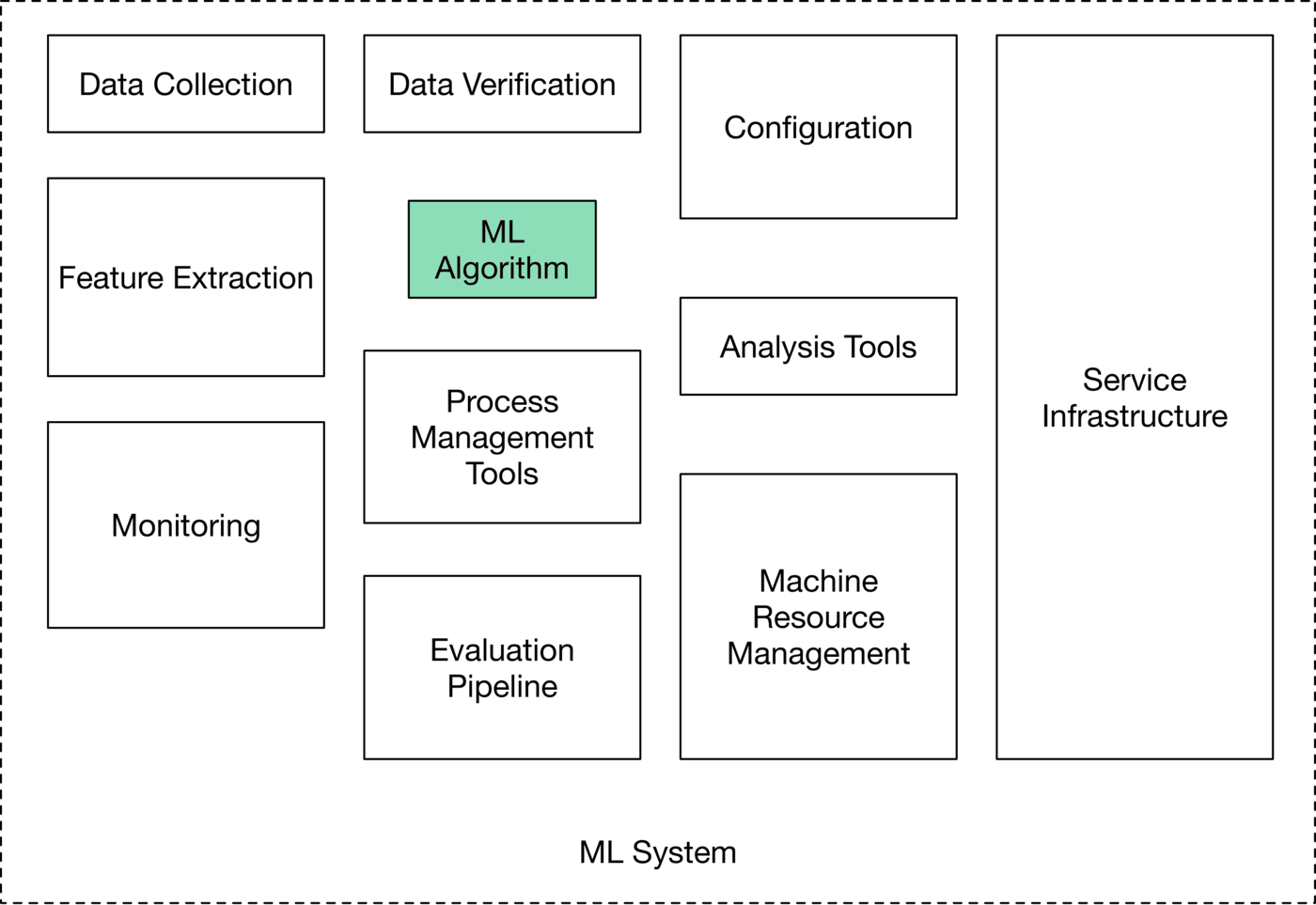
Many engineers think of ML algorithms such as logistic regression or neural networks as the entirety of an ML system. However, an ML system in production involves much more than just model development. ML systems are typically complex, consisting of a number of components, including data stacks to manage data, serving infrastructure to make the system available to millions of users, an evaluation pipeline to measure the performance of the proposed system, and monitoring to ensure the model's performance doesn't degrade over time.

At an ML system design interview, you are expected to answer open-ended questions. For example, you might be asked to design a movie recommendation system or a video search engine. There is no single correct answer. The interviewer wants to evaluate your thought process, your in-depth understanding of various ML topics, your ability to design an end-to-end system, and your design choices based on the trade-offs of various options.

To succeed in designing complex ML systems, it is very important to follow a framework. Unstructured answers make the flow difficult to follow. In this introduction, we propose a framework that is used throughout this book to tackle questions about ML system design. The framework consists of the following key steps:

1. Clarifying requirements
2. Framing the problem as an ML task
3. Data preparation
4. Model development
5. Evaluation
6. Deployment and serving
7. Monitoring and infrastructure

Every ML system design interview is different because the problem is open-ended, and there’s no one-size-fits-all way to succeed. The framework is intended to help you structure your thoughts, but there’s no need to follow it strictly. Be flexible. If an interviewer is mainly interested in model development, you should almost always adhere to their focus.

Let’s start by going over each step in the framework.

Clarifying Requirements

ML system design questions are usually intentionally vague, with the bare minimum of information. For example, an interview question could be: "design an event recommendation system". The first step is to ask clarifying questions. But what kind of questions to ask? Well, we should ask questions to understand the exact requirements. Here is a list of categorized questions to help us get started:

• Business objective. If we are asked to create a system to recommend vacation rentals, two possible motivations are to increase the number of bookings and increase the revenue.

• Features the system needs to support. What are some of the features that the system is expected to support which could affect our ML system design? For example, let’s assume we’re asked to design a video recommendation system. We might want to know if users can “like” or “dislike” recommended videos, as those interactions could be used to label training data.

• Data. What are the data sources? How large is the dataset? Is the data labeled?

• Constraints. How much computing power is available? Is it a cloud-based system, or should the system work on a device? Is the model expected to improve automatically over time?

• Scale of the system. How many users do we have? How many items, such as videos, are we dealing with? What’s the rate of growth of these metrics?

• Performance. How fast must prediction be? Is a real-time solution expected? Does accuracy have more priority or latency?

This list is not exhaustive, but you can use it as a starting point. Remember that other topics, such as privacy and ethics, can also be important. At the end of this step, we’re expected to reach an agreement with the interviewer about the scope and requirements of the system. It’s generally a good idea to write down the list of requirements and constraints we gather. By doing so, we ensure everyone is on the same page.

Frame the Problem as an ML Task

Effective problem framing plays a critical role in solving ML problems. Suppose an interviewer asks you to increase the user engagement of a video streaming platform. Lack of user engagement is certainly a problem, but it’s not an ML task. So, we should frame it as an ML task in order to solve it. In reality, we should first determine whether or not ML is necessary for solving a given problem. In an ML system design interview, it’s safe to assume that ML is helpful. So, we can frame the problem as an ML task by doing the following:

• Defining the ML objective
• Specifying the system’s input and output
• Choosing the right ML category

Defining the ML objective

A business objective can be to increase sales by 20% or to improve user retention. But the objective may not be well defined, and we cannot train a model simply by telling it, “increase sales by 20%”. For an ML system to solve a task, we need to translate the business objective into a well-defined ML objective. A good ML objective is one that ML models can solve. Let’s look at some examples as shown in Table 1.1. In later chapters, we will see more examples.

Table 1.1: Translate the business objective to an ML objective

Specifying the system’s input and output

Once we decide on the ML objective, we need to define the system’s inputs and outputs. For example, for a harmful content detection system on a social media platform, the input is a post, and the output is whether this post is considered harmful or not.

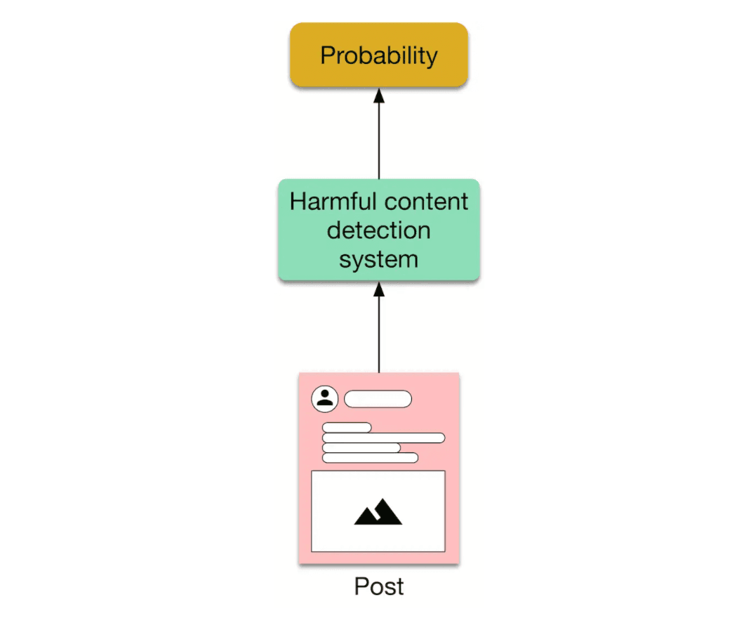
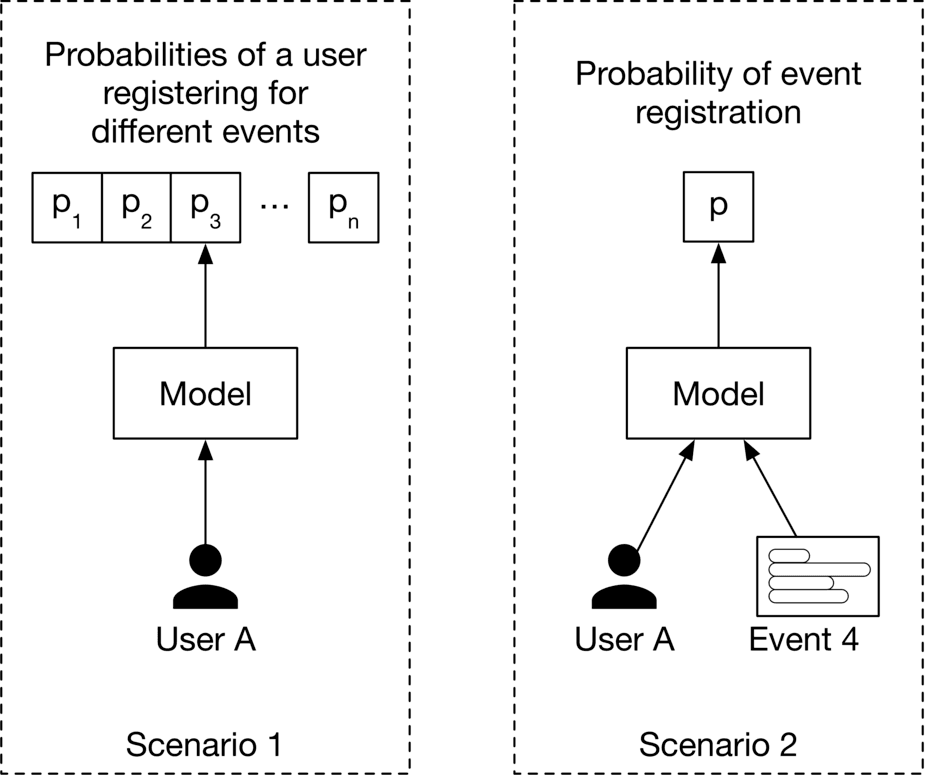
In some cases, the system may consist of more than one ML model. If so, we need to specify the input and output of each ML model. For example, for harmful content detection, we may want to use one model to predict violence and another model to predict nudity. The system depends on these two models to determine if a post is harmful or not.

Another important consideration is that there might be multiple ways to specify each model’s input-output. Figure 1.4 shows an example.

Choosing the right ML category

There are many different ways to frame a problem as an ML task. Most problems can be framed as one of the ML categories (leaf nodes) shown in Figure 1.5. As most readers are likely already familiar with them, we only provide an outline here.

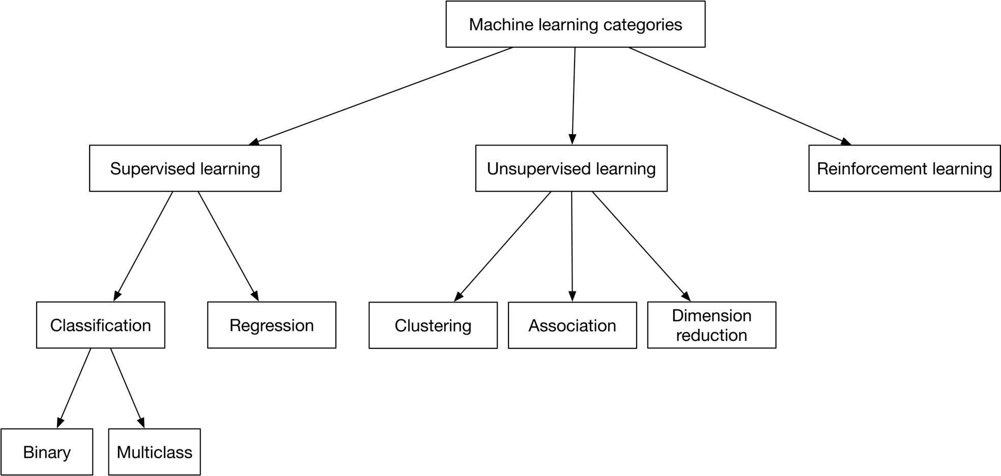
Supervised learning. A supervised learning model learns a task by using a training dataset. In reality, many problems fall into this category, since learning from a labeled dataset usually leads to better results.

Unsupervised learning. Unsupervised learning models make predictions by processing data that contain no correct answers. The goal of an unsupervised learning model

Reinforcement learning. In reinforcement learning, a computer agent learns to perform a task through repeated trial-and-error interactions with the environment. For example, robots can be trained to walk around a room using reinforcement learning, and software programs like AlphaGo can compete in the game of Go by using reinforcement learning.

Compared to supervised learning, unsupervised learning and reinforcement learning are less popular in real-world systems, as ML models usually learn a specific task better when training data is available. As a result, the majority of problems we tackle in this book rely on supervised learning. Let’s take a closer look at the different categories of supervised learning.

Classification model. Classification is the task of predicting a discrete class label; for example, whether an input image should be classified as "dog", "cat", or "rabbit". Classification models can be divided into two groups:

• Binary classification models predict a binary outcome. For example, the model predicts whether an image contains a dog or not

• Multiclass classification models classify the input into more than one class. For example, we can classify an image as a dog, cat, or rabbit

In this step, you are expected to choose the correct ML category. Later chapters provide examples of how to choose the right category during an interview.

Talking points

Here are some topics we might want to talk about during an interview:

• What is a good ML objective? How do different ML objectives compare? What are the pros and cons?
• What are the inputs and outputs of the system, given the ML objective?
• If more than one model is involved in the ML system, what are the inputs and outputs of each model?
• Does the task need to be learned in a supervised or unsupervised way?
• Is it better to solve the problem using a regression or classification model? In the case of classification, is it binary or multiclass? In the case of regression, what is the output range?

Data Preparation

ML models learn directly from data, meaning that data with predictive power is essential for training an ML model. This section aims to prepare high-quality inputs for ML models via two essential processes: data engineering and feature engineering. We will cover the important aspects of each process.

Data engineering

Data engineering is the practice of designing and building pipelines for collecting, storing, retrieving, and processing data. Let's briefly review data engineering fundamentals to understand the core components we may need.

Data sources

An ML system can work with data from many different sources. Knowing the data sources is a good way to answer many context questions, which may include: who collected it? How clean is the data? Can the data source be trusted? Is the data user-generated or system generated?

Data storage

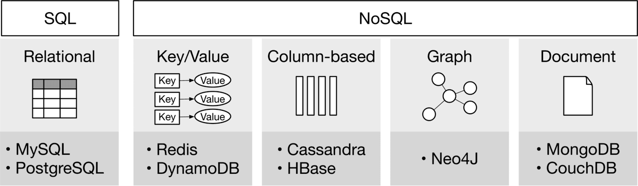
Data storage, also called a database, is a repository for persistently storing and managing collections of data. Different databases are built to satisfy different use cases, so it’s important to understand at a high level how different databases work. You are usually not expected to know database internals during ML system design interviews.

Extract, transform, and load (ETL)

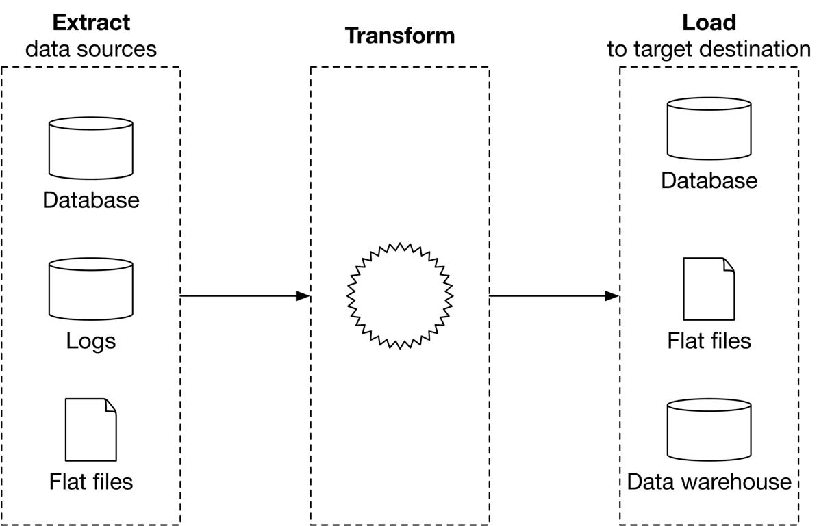
ETL consists of three phases:

• Extract. This process extracts data from different data sources.
• Transform. In this phase, data is often cleansed, mapped, and transformed into a specific format to meet operational needs.
• Load. The transformed data is loaded into the target destination, which can be a file, a database, or a data warehouse [1].

Data types

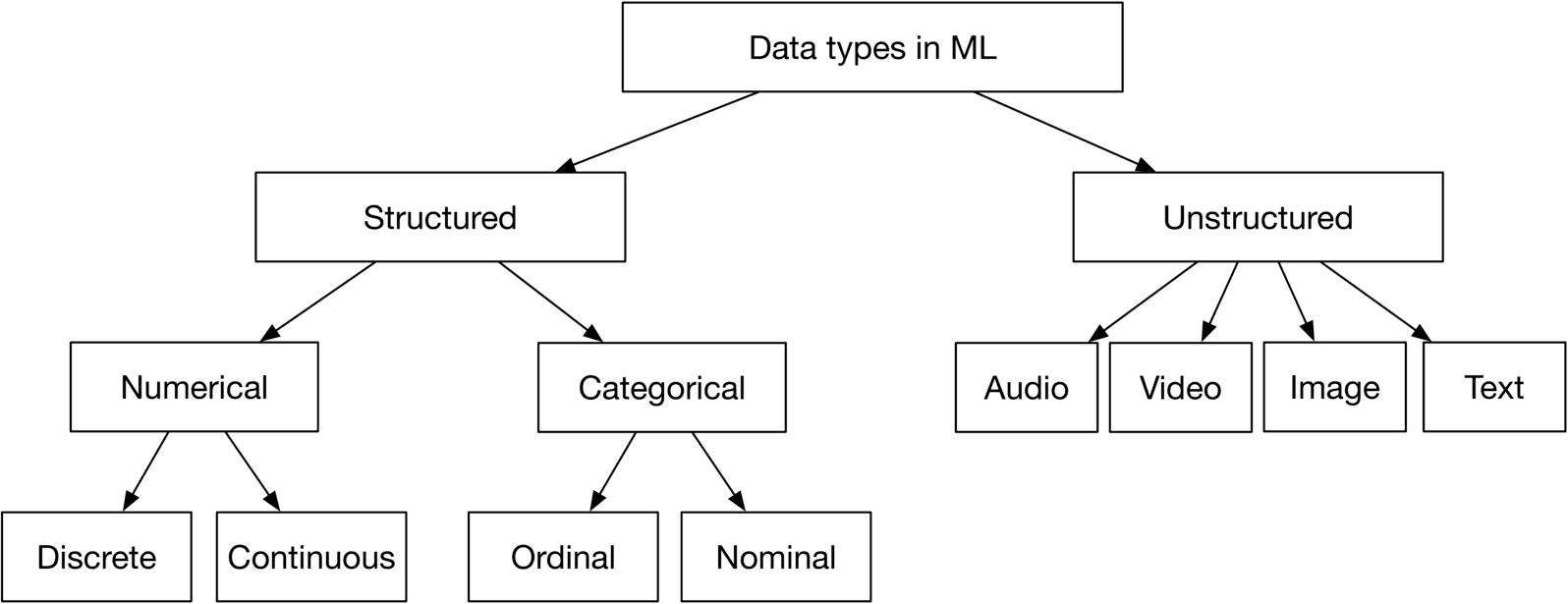
In ML, data types differ from those in programming languages, such as int, float, string, etc. At the high level, data types can be broken down into two types: structured and unstructured data, as shown in Figure 1.9.

Structured data follows a predefined data schema, whereas unstructured data does not. For example, dates, names, addresses, credit card numbers, and anything that can be represented in a tabular format with rows and columns, can be considered structured data. Unstructured data refers to data with no underlying data schema, such as images, audio files, videos, and text. Table 1.2 summarizes the key differences between structured and unstructured data.

Table 1.2: Summary of structured and unstructured data

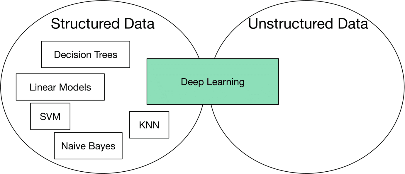
As shown in Figure 1.10, ML models perform differently based on the type of data. Understanding and clarifying whether the data is structured or unstructured helps us choose the appropriate ML model during the model development step.

Numerical data

Numerical data are any data points represented by numbers. As shown in Figure 1.9, numerical data is divided into continuous numerical data and discrete numerical data. For example, house prices can be considered as a continuous numerical value since a house price can take any value within a range. In contrast, the number of houses sold in the past year can be considered discrete numerical data, since it takes distinct values only.

Categorical data

Categorical data refers to data that can be stored and identified based on their assigned names or labels. For example, gender is categorical data since its value is from a limited set of age ranges. Categorical data can be divided into two groups: nominal and ordinal.

Nominal data refers to data with no numerical relationship between its categories. For example, gender is nominal data since there is no relationship between "male" and "female". Ordinal data refers to data with a predetermined or sequential order. For example, rating data which takes three unique values from "not happy", "neutral", and "happy" is an example of ordinal data.

Feature Engineering

Feature engineering contains two processes:

• Using domain knowledge to select and extract predictive features from raw data
• Transforming predictive features into a format usable by the model

Choosing the appropriate features is one of the most important decisions when developing and training ML models. It’s essential to choose features that bring the most value, and this feature engineering process requires subject matter expertise and is also highly dependent upon the task at hand. To help you master this process, we give many examples throughout this book.

Once the predictive features are chosen, they need to be transformed into suitable formats using feature engineering operations, which we examine next.

Feature engineering operations

It’s quite common for some of the selected features to not be in a format the model can use. Feature engineering operations transform the selected features into a format the model can use. Techniques include handling missing values, scaling values that have skewed distributions, and encoding categorical features. The following list is not comprehensive, but it contains some of the most common operations for structured data.

Handling missing values

Data in production often has missing values, which can generally be addressed in two ways: deletion or imputation.

Deletion. This method removes any records with a missing value in any of the features. Deletion can be divided into row deletion and column deletion. In column deletion, we remove the whole column representing a feature, if the feature has too many missing values. In row deletion, we remove a row representing a data point if the data point has many missing values.

The drawback of deletion is that it reduces the quantity of data the model can potentially use for training. This is not ideal since ML models tend to work better when they are exposed to more data.

Imputation. Alternatively, we can impute the missing values by filling them with certain values. Some common practices include:

• Filling in missing values with their defaults
• Filling in missing values with the mean, median, or mode (the most common value)

The drawback of imputation is it may introduce noise to the data. It’s important to note that no technique is perfect for handling missing values, as each has its trade-offs

Feature scaling

Feature scaling refers to the process of scaling features to have a standard range and distribution. Let’s first look at why feature scaling might be needed.

Many ML models struggle to learn a task when the features of the dataset are in different ranges. For example, features such as age and income might have different value ranges. In addition, some models may struggle to learn the task when a feature has a skewed distribution. What are some of the feature scaling techniques? Let’s take a look.

Normalization (min-max scaling). In this approach, the features are scaled, so all values are within the range $[0, 1]$ using the following formula:

Note that normalization does not change the distribution of the feature. In order to change the distribution of a feature to follow a standard distribution, standardization is used.

Standardization (Z-score normalization). Standardization is the process of changing the distribution of a feature to have a $0$ mean and a standard deviation of $1$. The following formula is used to standardize a feature:

Where $\mu$ is the feature’s mean and $\sigma$ is the standard deviation.

Log scaling. To mitigate the skewness of a feature, a common technique called log scaling can be used, with the following formula:

Log transformation can make data distribution less skewed, and enable the optimization algorithm to converge faster.

Discretization (Bucketing)

Discretization is the process of converting a continuous feature into a categorical feature. For example, instead of representing height as a continuous feature, we can divide heights into discrete buckets and represent each height by the bucket to which it belongs. This allows the model to focus on learning only a few categories instead of attempting to learn an infinite number of possibilities.

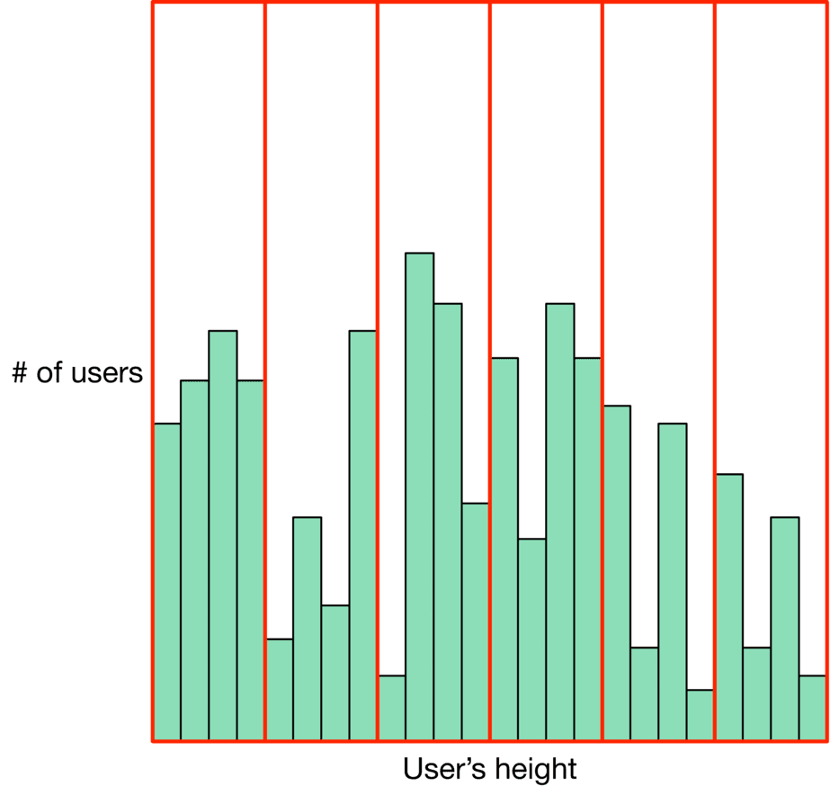
Discretization can also be applied to discrete features. For example, a user’s age is a discrete feature, but discretizing it reduces the number of categories, as shown in Table 1.3.

Table 1.3: Discretizing numeric age attributes

Encoding categorical features

In most ML models, all inputs and outputs must be numerical. This means if a feature is categorical, we should encode it into numbers before sending it to the model. There are three common methods for converting categorical features into numeric representations: integer encoding, one-hot encoding, and embedding learning.

Integer encoding. An integer value is assigned to each unique category value. For example, “Excellent” is $1$, “Good” is $2$, and “Bad” is $3$. This method is useful if the integer values have a natural relationship with each other.

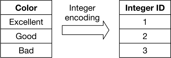
However, when there is no ordinal relationship between categorical features, integer encoding is not a good choice. One-hot encoding, which we will examine next, addresses this issue.

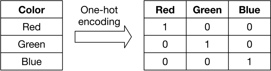
One-hot encoding. With this technique, a new binary feature is created for each unique value. As shown in Figure 1.14, we replace the original feature (color) with three new binary features (red, green, and blue). For example, if a data point has a “red” color, we replace it with “$1$, $0$, $0$”.

Embedding learning. Another way to encode a categorical feature is to use embedding learning. An embedding is a mapping of a categorical feature into an $N$-dimensional vector. Embedding learning is the process of learning an N-dimensional vector for each unique value that the categorical feature may take. This approach is useful when the number of unique values the feature takes is very large. In this case, one-hot encoding is not a good option because it leads to very large vector sizes. We will see more examples in later chapters.

Talking points

Here are some topics we might want to discuss during the interview:

• Data availability and data collection: What are the data sources? What data is available to us, and how do we collect it? How large is the data size? How often do new data come in?
• Data storage: Where is the data currently stored? Is it on the cloud or on user devices? Which data format is appropriate for storing the data? How do we store multimodal data, e.g., a data point that might contain both images and texts?
• Feature engineering: How do we process raw data into a form that’s useful for the models? What should we do about missing data? Is feature engineering required for this task? Which operations do we use to transform the raw data into a format usable by the ML model? Do we need to normalize the features? Which features should we construct from the raw data? How do we plan to combine data of different types, such as texts, numbers, and images?
• Privacy: How sensitive are the available data? Are users concerned about the privacy of their data? Is anonymization of user data necessary? Is it possible to store users’ data on our servers, or is it only possible to access their data on their devices?
• Biases: Are there any biases in the data? If yes, what kinds of biases are present, and how do we correct them?

Model Development

Model development refers to the process of selecting an appropriate ML model and training it to solve the task at hand.

Model selection

Model selection is the process of choosing the best ML algorithm and architecture for a predictive modeling problem. In practice, a typical process for selecting a model is to:

• Establish a simple baseline. For example, in a video recommendation system, the baseline can be obtained by recommending the most popular videos.
• Experiment with simple models. After we have a baseline, a good practice is to explore ML algorithms that are quick to train, such as logistic regression.
• Switch to more complex models. If simple models cannot deliver satisfactory results, we can then consider more complex models, such as deep neural networks.
• Use an ensemble of models if we want more accurate predictions. Using an ensemble of multiple models instead of only one may improve the quality of predictions. Creating an ensemble can be accomplished in three ways: bagging [2], boosting [3], and stacking [4], which will be discussed in later chapters.

In an interview setting, it’s important to explore various model options and discuss their pros and cons. Some typical model options include:

• Logistic regression
• Linear regression
• Decision trees
• Gradient boosted decision trees and random forests
• Support vector machines
• Naive Bayes
• Factorization Machines (FM)
• Neural networks

When examining different options, it’s good to briefly explain the algorithm and discuss the trade-offs. For example, logistic regression may be a good option for learning a linear task, but if the task is complex, we may need to choose a different model. When choosing an ML algorithm, it’s important to consider different aspects of a model. For example:

• The amount of data the model needs to train on
• Training speed
• Hyperparameters to choose and hyperparameter tuning techniques
• Possibility of continual learning
• Compute requirements. A more complex model might deliver higher accuracy, but might require more computing power, such as a GPU instead of a CPU
• Model’s interpretability [5]. A more complex model can give better performance, but its results may be less interpretable

There is no single best algorithm that solves all problems. The interviewer wants to see if you have a good understanding of different ML algorithms, their pros and cons, and your ability to choose a model based on requirements and constraints. To help you improve model selection, this book contains a variety of model selection examples. This book assumes you are familiar with common ML algorithms. To refresh your memory, read [6].

Model training

Once the model selection is complete, it’s time to train the model. During this step, there are various topics you may want to discuss at an interview, such as:

• Constructing the dataset
• Choosing the loss function
• Training from scratch vs. fine-tuning
• Distributed training

Let’s look at each one.

Constructing the dataset

At an interview, it’s usually a good idea to talk about constructing the dataset for model training and evaluation. As Figure 1.15 illustrates, there are 5 steps in constructing the dataset.

All the steps except “identify features and labels” are generic operations, which can be applied to any ML system design task. In this chapter, we will take a close look at each step, but in later chapters, we will mainly focus on “identify features and labels,” which is task-specific.

Collect the raw data

This is extensively discussed in the data preparation step, so we do not repeat it here.

Identify features and labels

During the feature engineering step, we have already discussed which features to use. So, let’s focus on creating labels for the data. There are two common ways to get labels: hand labeling and natural labeling.

Hand labeling. This means individual annotators label the data by hand. For example, an individual annotator labels whether a post contains misinformation or not. Hand labeling leads to accurate labels since a human is involved in the process. However, hand labeling has many drawbacks; it is expensive and slow, introduces bias, requires domain knowledge, and is a threat to data privacy.

Natural labeling. In natural labeling, the ground truth labels are inferred automatically without human annotations. Let’s see an example to better understand natural labels.

Suppose we want to design an ML system that ranks news feeds based on relevance. One possible way to solve this task is to train a model which takes a user and a post as input, and outputs the probability that the user will press the ``like” button after seeing this post. In this case, the training data are pairs of $\langle$ user, post $\rangle$ and their corresponding label, which is 1 if the user liked the post, and 0 if they did not. This way, we are able to naturally label the training data without relying on human annotations.

In this step, it is important to clearly communicate how we obtain training labels and what the training data looks like.

Select a sampling strategy

It is often impractical to collect all the data, so sampling is an efficient way to reduce the amount of data in the system. Common sampling strategies include convenience sampling, snowball sampling, stratified sampling, reservoir sampling, and importance sampling. To learn more about sampling methods, you can refer to [7].

Split the data

Data splitting refers to the process of dividing the dataset into training, evaluation (validation), and test dataset. To learn more about data splitting techniques, refer to [8].

Address any class imbalances

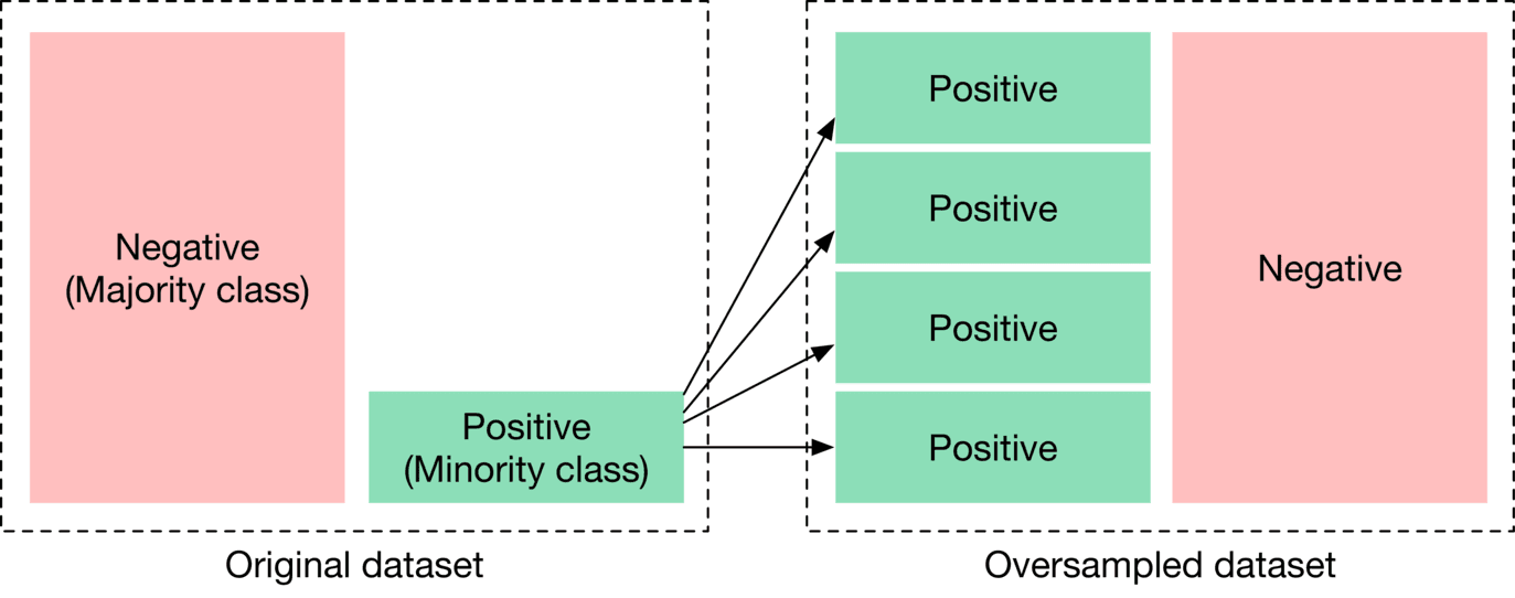
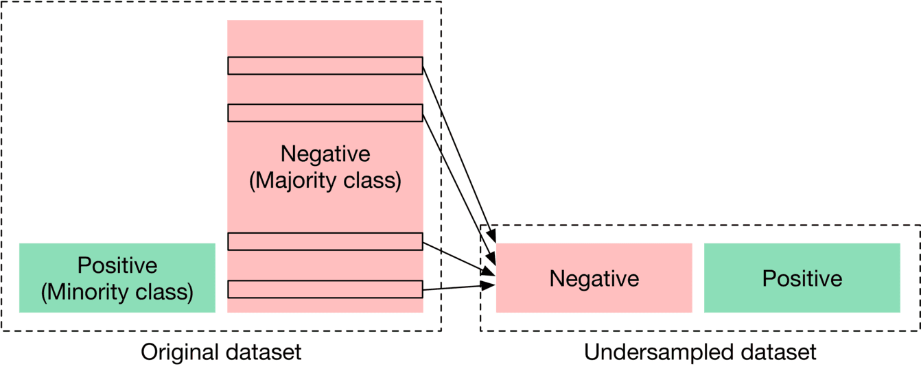
A dataset with skewed class labels is called an imbalanced dataset. The class that makes up a larger proportion of the dataset is called the majority class, and the class which comprises a smaller proportion of the dataset is known as the minority class.

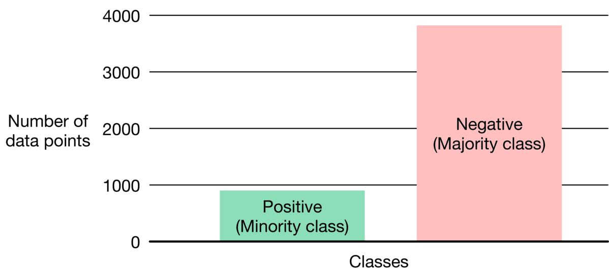
An imbalanced dataset is a serious issue in model training, as it means a model may not have enough data to learn the minority class. There are different techniques to mitigate this issue. Let’s take a look at two commonly used approaches: resampling training data and altering the loss function.

Resampling training data

Resampling refers to the process of adjusting the ratio between different classes, making the data more balanced. For example, we can oversample the minority class (Figure 1.17) or undersample the majority class (Figure 1.18)

Altering the loss function

This technique alters the loss function to make it more robust against class imbalance. The high-level idea is to give more weight to data points from the minority class. A higher weight in the loss function penalizes the model more when it makes a wrong prediction about a minority class. This forces the model to learn minority classes more effectively. Two commonly used loss functions to mitigate class imbalance are class-balanced loss [9] and focal loss [10][11].

Choosing the loss function

Once the dataset is constructed, we need to choose a proper loss function to train the model. A loss function is a measurement of how accurate the model is at predicting an expected outcome. The loss function allows the optimization algorithm to update the model’s parameters during the training process in order to minimize the loss.

Designing a novel loss function is not easy. In ML interviews, you are usually expected to select a loss function from a list of existing loss functions based on how you framed the problem. Sometimes, you might need to make minor changes to the loss function to make it specific to the problem. We will provide more examples in later chapters.

Training from scratch vs. fine-tuning

One topic that might be useful to discuss briefly is training from scratch vs. fine-tuning. Fine-tuning means continuing to train the model on new data by making small changes to its learned parameters. This is a design decision you may need to discuss with the interviewer.

Distributed training

Training at scale becomes increasingly important because models grow bigger over time, and the size of the dataset also increases dramatically. Distributed training is commonly used to train the model, by dividing the work among multiple worker nodes. These worker nodes operate in parallel in order to speed up model training. There are two main types of distributed training: data parallelism [12] and model parallelism [13].

Depending on which task we are solving, employing distributed training may be necessary. In such cases, it’s important to discuss this topic with the interviewer. Note that distributed training is a generic topic you can talk about irrespective of the specific task.

Talking points

Some talking points are listed below:

• Model selection: Which ML models are suitable for the task, and what are their pros and cons. Here’s a list of topics to consider during model selection:
  • The time it takes to train
  • The amount of training data the model expects
  • The computing resources the model may need
  • Latency of the model at inference time
  • Can the model be deployed on a user’s device?
  • Model’s interpretability. Making a model more complex may increase its performance, but the results might be harder to interpret
  • Can we leverage continual training, or should we train from scratch?
  • How many parameters does the model have? How much memory is needed?
  • For neural networks, you might want to discuss typical architectures/blocks, such as ResNet or Transformer-based architectures. You can also discuss the choice of hyperparameters, such as the number of hidden layers, the number of neurons, activation functions, etc.
• Dataset labels: How should we obtain the labels? Is the data annotated, and if so, how good are the annotations? If natural labels are available, how do we get them? How do we receive user feedback on the system? How long does it take to get natural labels?
• Model training.
  • What loss function should we choose? (e.g., Cross-entropy [14], MSE [15], MAE [16], Huber loss [17], etc.)
  • What regularization should we use? (e.g., L1 [19], L2 [18], Entropy Regularization [19], K-fold CV [20], or dropout [21])
  • What is backpropagation?
  • You may need to describe common optimization methods such as SGD [22], AdaGrad [23], Momentum [24], and RMSProp [25].
  • What activation functions do we want to use and why? (e.g., ELU [26], ReLU [27], Tanh [28], Sigmoid [29]).
  • How to handle an imbalanced dataset?
  • What is the bias/variance trade-off?
  • What are the possible causes of overfitting and underfitting? How to address them?
• Continual learning: Do we want to train the model online with each new data point? Do we need to personalize the model to each user? How often do we retrain the model? Some models need to be retrained daily or weekly, and others monthly or yearly.

Evaluation

The next step after the model development is evaluation, which is the process of using different metrics to understand an ML model’s performance. In this section, we examine two evaluation methods, offline and online.

Offline evaluation

Offline evaluation refers to evaluating the performance of ML models during the model development phase. To evaluate a model, we usually first make predictions using the evaluation dataset. Next, we use various offline metrics to measure how close the predictions are to the ground truth values. Table 1.4 shows some of the commonly used metrics for different tasks.

Table 1.4: Popular metrics in offline evaluation

During an interview, it’s important to identify suitable metrics for offline evaluation. This depends on the task at hand and how we have framed it. For example, if we try to solve a ranking problem, we might need to discuss ranking metrics and their trade-offs.

Online evaluation

Online evaluation refers to the process of evaluating how the model performs in production after deployment. To measure the impact of the model, we need to define different metrics. Online metrics refer to those we use during an online evaluation and are usually tied to business objectives. Table 1.5 shows various metrics for different problems.

Table 1.5: Possible metrics in online evaluation

In practice, companies usually track many online metrics. At an interview, we need to select some of the most important ones to measure the impact of the system. As opposed to offline metrics, choosing online metrics Online metrics is subjective and depends upon product owners and business stakeholders.

In this step, the interviewer gauges your business sense. So, it is helpful to communicate your thought process and your reasons for choosing certain metrics.

Talking points

Here are some talking points for the evaluation step:

• Online metrics: Which metrics are important for measuring the effectiveness of the ML system online? How do these metrics relate to the business objective?
• Offline metrics: Which offline metrics are good at evaluating the model’s predictions during the development phase?
• Fairness and bias: Does the model have the potential for bias across different attributes such as age, gender, race, etc.? How would you fix this? What happens if someone with malicious intent gets access to your system?

Deployment and Serving

A natural next step after choosing the appropriate metrics for online and offline evaluations is to deploy the model to production and serve millions of users. Some important topics to cover include:

• Cloud vs. on-device deployment
• Model compression
• Testing in production
• Prediction pipeline

Let's take a look at each.

Cloud vs. on-device deployment

Deploying a model on the cloud is different from deploying it on a mobile device. Table 1.6 summarizes the main differences between on-device deployment and cloud deployment.

Table 1.6: Trade-offs between cloud and on-device deployment

Model compression

Model compression refers to the process of making a model smaller. This is necessary to reduce the inference latency and model size. Three techniques are commonly used to compress models:

• Knowledge distillation: The goal of knowledge distillation is to train a small model (student) to mimic a larger model (teacher).
• Pruning: Pruning refers to the process of finding the least useful parameters and setting them to zero. This leads to sparser models which can be stored more efficiently.
• Quantization: Model parameters are often represented with 32-bit floating numbers. In quantization, we use fewer bits to represent the parameters, which reduces the model’s size. Quantization can happen during training or post-training [37].

To learn more about model compression, you are encouraged to read [38].

Test in production

The only way to ensure the model will perform well in production is to test it with real traffic. Commonly used techniques to test models include shadow deployment [39], A/B testing [40], canary release [41], interleaving experiments [42], bandits [43], etc.

To demonstrate that we understand how to test in production, it’s a good idea to mention at least one of these methods. Let’s briefly review shadow deployment and A/B testing.

Shadow deployment

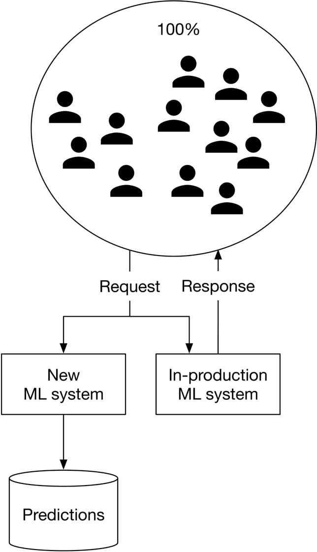
In this method, we deploy the new model in parallel with the existing model. Each incoming request is routed to both models, but only the existing model's prediction is served to the user.

By shadow deploying the model, we minimize the risk of unreliable predictions until the newly developed model has been thoroughly tested. However, this is a costly approach that doubles the number of predictions.

A/B testing

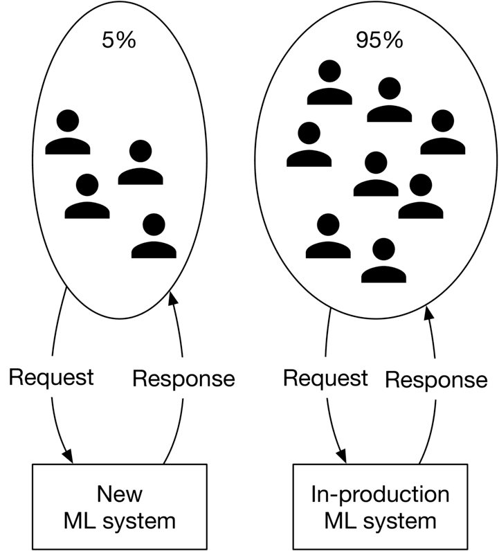
With this method, we deploy the new model in parallel with the existing model. A portion of the traffic is routed to the newly developed model, while the remaining requests are routed to the existing model.

In order to execute A/B testing correctly, there are two important factors to consider. First, the traffic routed to each model has to be random. Second, A/B tests should be run on a sufficient number of data points in order for the results to be legitimate.

Prediction pipeline

To serve requests in production, we need a prediction pipeline. An important design decision to make is the choice between online prediction and batch prediction.

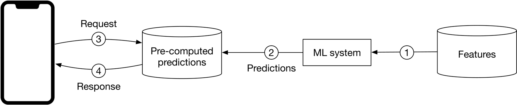
Batch prediction. With batch prediction, the model makes predictions periodically. Because predictions are pre-computed, we don’t need to worry about how long it takes the model to generate predictions once they are pre-computed.

However, the batch prediction has two major drawbacks. First, the model becomes less responsive to the changing preferences of users. Secondly, batch prediction is only possible if we know in advance what needs to be pre-computed. For example, in a language translation system, we are not able to make translations in advance as it entirely depends on the user’s input.

Online prediction. In online prediction, predictions are generated and returned as soon as requests arrive. The main problem with online prediction is that the model might take too long to generate predictions.

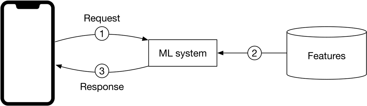
This choice of batch prediction or online prediction is mainly driven by product requirements. Online prediction is generally preferred in situations where we do not know what needs to be computed in advance. Batch prediction is ideal when the system processes a high volume of data, and the results are not needed in real time.

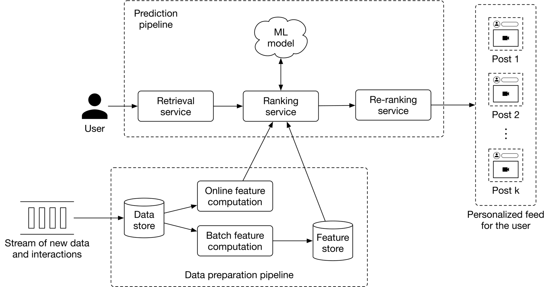
As previously discussed, ML system development involves more than just ML modeling. Proposing an overall ML system design in an interview demonstrates a deep understanding of how different components work together as a whole. Interviewers often take this as a critical signal.

Figure 1.23 shows an example of the ML system design for a personalized news feed system. We will examine it in more depth in Chapter 10.

Talking points

• Is model compression needed? What are some commonly used compression techniques?
• Is online prediction or batch prediction more suitable? What are the trade-offs?
• Is real-time access to features possible? What are the challenges?
• How should we test the deployed model in production?
• An ML system consists of various components working together to serve requests. What are the responsibilities of each component in the proposed design?
• What technologies should we use to ensure that serving is fast and scalable?

Monitoring

Monitoring refers to the task of tracking, measuring, and logging different metrics. An ML system in production can fail for many reasons. Monitoring helps to detect system failures when they occur, so they can be fixed as quickly as possible.

Monitoring is an important topic to discuss in ML system design interviews. Two primary areas you may want to discuss are:

• Why a system fails in production
• What to monitor

Why a system fails in production

There are various reasons why an ML system may fail after it is deployed to production. One of the most common reasons is data distribution shift.

Data distribution shift refers to the scenario in which the data a model encounters in production differs from that it encountered during training. Figure 1.24 shows an example where the training data comprised images of cups seen from the front view, but at serving time, an image of a cup at a different angle is passed to the ML model.

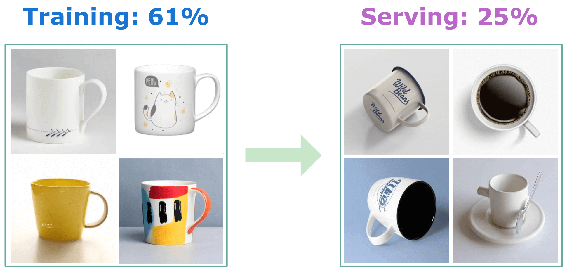
Data distribution in the real world constantly changes. In other words, the data used for training is likely to become less relevant as time passes. This leads to a stale model with deteriorating performance over time. Therefore, we should continuously monitor the system to detect this problem. Two common approaches for dealing with data distribution shifts are:

• Train on large datasets. A big enough training dataset enables the model to learn a comprehensive distribution, so any data points encountered in production likely come from this learned distribution.
• Regularly retrain the model using labeled data from the new distribution.

What to monitor

This is a broad topic, and here we focus on post-production monitoring techniques. Our goal is to detect failures and identify shifts in the ML system. Broadly speaking, we can categorize monitoring techniques in ML systems into two buckets: operation-related and ML-specific metrics.

Operation-related metrics: Those metrics ensure the system is up and running. They include average serving times, throughput, the number of prediction requests, CPU/GPU utilization, etc.

ML-specific metrics:

• Monitoring inputs/outputs. Models are only as good as the data they consume, so monitoring the model’s input and outputs is vital.
• Drifts. Inputs to the system and the model’s outputs are monitored to detect changes in their underlying distribution.
• Model accuracy. For example, we expect the accuracy to be within a specific range.
• Model versions. Monitor which version of the model is deployed.

Infrastructure

Infrastructure is the foundation for training, deploying, and maintaining ML systems.

In many ML interviews, you won’t be asked infrastructure-related questions. However, some ML roles, such as DevOps and MLOps may require infrastructure knowledge. So, it’s important to be clear about the interviewer’s expectations for this topic.

Infrastructure is a very broad subject and cannot be summarized in just a few lines. If you’re interested in learning more about ML infrastructure, refer to [44][45][46].

Summary

In this chapter, we proposed a framework for an ML system design interview. While many topics discussed in this chapter are task-specific, some are generic and applicable to a wide range of tasks. Throughout this book, we only focus on unique talking points specific to the problem at hand, in order to avoid repetition. For example, topics related to deployment, monitoring, and infrastructure are often similar, regardless of the task. Therefore, we do not repeat generic topics in later chapters, but you are usually expected to talk about them during an interview.

Finally, no engineer can be an expert in every aspect of the ML lifecycle. Some engineers specialize in deployment and production, while others specialize in model development. Some companies may not care about infrastructure, while others may focus heavily on monitoring and infrastructure. Data science roles generally require more data engineering, while applied ML roles focus more on model development and productionization. Depending on the role and the interviewer's preference, some steps may be discussed in more detail, while others may be discussed briefly or even skipped. In general, a candidate should seek to drive the conversation, while being ready to go with the interviewer’s flow, if they raise a question.

Now you understand these fundamentals, we’re ready to tackle some of the most common ML system design interview questions.

References

1. Data warehouse. https://cloud.google.com/learn/what-is-a-data-warehouse.
2. Bagging technique in ensemble learning. https://en.wikipedia.org/wiki/Bootstrap_aggregating.
3. Boosting technique in ensemble learning. https://aws.amazon.com/what-is/boosting/.
4. Stacking technique in ensemble learning. https://machinelearningmastery.com/stacking-ensemble-machine-learning-with-python/.
5. Interpretability in Machine Mearning. https://blog.ml.cmu.edu/2020/08/31/6-interpretability/.
6. Traditional machine learning algorithms. https://machinelearningmastery.com/a-tour-of-machine-learning-algorithms/.
7. Sampling strategies. https://www.scribbr.com/methodology/sampling-methods/.
8. Data splitting techniques. https://machinelearningmastery.com/train-test-split-for-evaluating-machine-learning-algorithms/.
9. Class-balanced loss. https://arxiv.org/pdf/1901.05555.pdf.
10. Focal loss paper. https://arxiv.org/pdf/1708.02002.pdf.
11. Focal loss. https://medium.com/swlh/focal-loss-an-efficient-way-of-handling-class-imbalance-4855ae1db4cb.
12. Data parallelism. https://www.telesens.co/2017/12/25/understanding-data-parallelism-in-machine-learning/.
13. Model parallelism. https://docs.aws.amazon.com/sagemaker/latest/dg/model-parallel-intro.html.
14. Cross entropy loss. https://en.wikipedia.org/wiki/Cross_entropy.
15. Mean squared error loss. https://en.wikipedia.org/wiki/Mean_squared_error.
16. Mean absolute error loss. https://en.wikipedia.org/wiki/Mean_absolute_error.
17. Huber loss. https://en.wikipedia.org/wiki/Huber_loss.
18. L1 and l2 regularization. https://www.analyticssteps.com/blogs/l2-and-l1-regularization-machine-learning.
19. Entropy regularization. https://paperswithcode.com/method/entropy-regularization.
20. K-fold cross validation. https://en.wikipedia.org/wiki/Cross-validation_(statistics).
21. Dropout paper. https://jmlr.org/papers/volume15/srivastava14a/srivastava14a.pdf.
22. Stochastic gradient descent. https://en.wikipedia.org/wiki/Stochastic_gradient_descent.
23. AdaGrad optimization algorithm. https://optimization.cbe.cornell.edu/index.php?title=AdaGrad.
24. Momentum optimization algorithm. https://optimization.cbe.cornell.edu/index.php?title=Momentum.
25. RMSProp optimization algorithm. https://optimization.cbe.cornell.edu/index.php?title=RMSProp.
26. ELU activation function. https://ml-cheatsheet.readthedocs.io/en/latest/activation_functions.html#elu.
27. ReLU activation function. https://ml-cheatsheet.readthedocs.io/en/latest/activation_functions.html#relu.
28. Tanh activation function. https://ml-cheatsheet.readthedocs.io/en/latest/activation_functions.html#tanh.
29. Sigmoid activation function. https://ml-cheatsheet.readthedocs.io/en/latest/activation_functions.html#softmax.
30. FID score. https://en.wikipedia.org/wiki/Fr%C3%A9chet_inception_distance.
31. Inception score. https://en.wikipedia.org/wiki/Inception_score.
32. BLEU metrics. https://en.wikipedia.org/wiki/BLEU.
33. METEOR metrics. https://en.wikipedia.org/wiki/METEOR.
34. ROUGE score. https://en.wikipedia.org/wiki/ROUGE_(metric).
35. CIDEr score. https://arxiv.org/pdf/1411.5726.pdf.
36. SPICE score. https://arxiv.org/pdf/1607.08822.pdf.
37. Quantization-aware training. https://pytorch.org/docs/stable/quantization.html.
38. Model compression survey. https://arxiv.org/pdf/1710.09282.pdf.
39. Shadow deployment. https://christophergs.com/machine%20learning/2019/03/30/deploying-machine-learning-applications-in-shadow-mode/.
40. A/B testing. https://en.wikipedia.org/wiki/A/B_testing.
41. Canary release. https://blog.getambassador.io/cloud-native-patterns-canary-release-1cb8f82d371a.
42. Interleaving experiment. https://netflixtechblog.com/interleaving-in-online-experiments-at-netflix-a04ee392ec55.
43. Multi-armed bandit. https://vwo.com/blog/multi-armed-bandit-algorithm/.
44. ML infrastructure. https://www.run.ai/guides/machine-learning-engineering/machine-learning-infrastructure.
45. Interpretability in ML. https://fullstackdeeplearning.com/spring2021/lecture-6/.
46. Chip Huyen. Designing Machine Learning Systems: An Iterative Process for Production-Ready Application. ” O’Reilly Media, Inc.”, 2022.