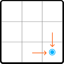
You are positioned at the top-left corner of a m × n matrix, and can only move downward or rightward through the matrix. Determine the number of unique pathways you can take to reach the bottom-right corner of the matrix.

Example:

Input: m = 3, n = 3
Output: 6

Constraints:

• m, n ≥ 1

In Plain English

New to this one? Start here. Below is the core idea in everyday language, plus a real-world analogy—then the sections that follow build on it with the formal reasoning, code, and step-by-step walkthroughs.

Intuition

At each cell, we can either move right or move down. No matter which direction we choose at any point, it will always move us closer to the destination. This means we just need to keep moving either right or down until we can no longer do so, at which point we’ve reached the bottom-right corner.

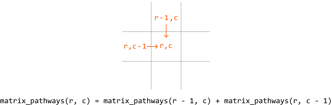
Let's think about this problem backward. Assume we have already reached the bottom-right corner. How did we get here? We know for certain we came from either the cell directly above, or the cell directly to the left of the current position.

This is equally true for any cell on the matrix, which means a generalization can be made: the number of paths to any cell is equal to the sum of the number of paths to the cell above it and the cell to its left.

This demonstrates the existence of subproblems, and that this problem has an optimal substructure, where we need to solve two subproblems in order to solve the main problem. This makes this problem well-suited for DP. So, let’s translate the above recurrence relation to a DP formula:

dp[r][c] = dp[r - 1][c] + dp[r][c - 1], where dp[r][c] represents the total number of paths that lead to cell (r, c).

Before populating the DP table, we need to know our base cases.

Base cases
We know dp[0][0] should be 1 because there’s only one path leading to cell (0, 0).

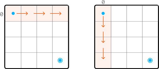
What else do we know for certain? Since we can only move right or down, once we leave a row or column, we can never return to it because we can't move left or up. This means, for any cell in row 0 or column 0, there’s only one path to those cells:

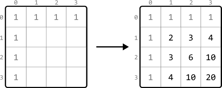
Therefore, we can set all cells in row 0 and column 0 to 1 as the base cases.

Problem-solving tip: another way to identify row 0 and column 0 as base cases is by examining the DP formula. Since we need the values from row r - 1 and column c - 1 to populate dp[r][c], all values at r = 0 and c = 0 must be pre-populated before using the formula to avoid index out-of-bound errors.

Populating the DP table
Once the base cases are set, we can populate the remaining DP table, starting from cell (1, 1), using our DP formula (dp[r][c] = dp[r-1][c] + dp[r][c-1]):

After we fill in the DP table, we can return dp[m - 1][n - 1], which contains the number of paths to the bottom-right corner.

Implementation

def matrix_pathways(m: int, n: int) -> int:
    # Base cases: Set all cells in row 0 and column 0 to 1. We can do this by
    # initializing all cells in the DP table to 1.
    dp = [[1] * n for _ in range(m)]
    # Fill in the rest of the DP table.
    for r in range(1, m):
        for c in range(1, n):
            # Paths to current cell = paths from above + paths from left.
            dp[r][c] = dp[r - 1][c] + dp[r][c - 1]
    return dp[m - 1][n - 1]

#include <vector>
using namespace std;

long long matrixPathways(int m, int n) {
    // Start every cell at 1: this handles row 0 and column 0 (one way each).
    vector<vector<long long>> dp(m, vector<long long>(n, 1));
    for (int r = 1; r < m; r++) {
        for (int c = 1; c < n; c++) {
            // Paths to this cell = paths from above + paths from the left.
            dp[r][c] = dp[r - 1][c] + dp[r][c - 1];
        }
    }
    return dp[m - 1][n - 1];
}

// These methods live inside a class, e.g. class Solution { ... }
long matrixPathways(int m, int n) {
    // Start every cell at 1: this handles row 0 and column 0 (one way each).
    long[][] dp = new long[m][n];
    for (long[] row : dp) Arrays.fill(row, 1);
    for (int r = 1; r < m; r++) {
        for (int c = 1; c < n; c++) {
            // Paths to this cell = paths from above + paths from the left.
            dp[r][c] = dp[r - 1][c] + dp[r][c - 1];
        }
    }
    return dp[m - 1][n - 1];
}

Complexity Analysis

Time complexity: The time complexity of matrix_pathways is $O(m\cdot n)$ because each cell in the DP table is populated once.

Space complexity: The space complexity is $O(m\cdot n)$ due to the DP table, which contains $m\cdot n$ elements.

Optimization

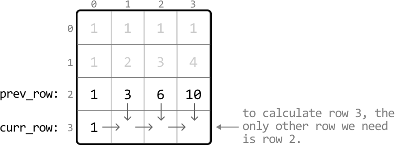
We can optimize our solution by understanding that, for each cell in the DP table, we only need to access the cells directly above it and to its left.

• To get the cell above it (dp[r-1][c]), we only need access to the previous row.
• To get the cell to its left (dp[r][c-1]), we just need to look at the cell to the left of the current cell, which is in the same row we're currently populating.

Therefore, we only need to maintain two rows:

• prev_row: the previous row.
• curr_row: the current row being populated.

This effectively reduces the space complexity to $O(n)$ because we now only need to maintain two arrays of size $n$. After populating the DP values for the current row, we’ll need to make sure to update prev_row with the values from curr_row to prepare for the next iteration since the next row’s previous row is the current row. Below is the optimized code:

def matrix_pathways_optimized(m: int, n: int) -> int:
    # Initialize 'prev_row' as the DP values of row 0, which are all 1s.
    prev_row = [1] * n
    # Iterate through the matrix starting from row 1.
    for r in range(1, m):
        # Set the first cell of 'curr_row' to 1. This is done by
        # setting the entire row to 1.
        curr_row = [1] * n
        for c in range(1, n):
            # The number of unique paths to the current cell is the sum
            # of the paths from the cell above it ('prev_row[c]') and
            # the cell to the left ('curr_row[c - 1]').
            curr_row[c] = prev_row[c] + curr_row[c - 1]
        # Update 'prev_row' with 'curr_row' values for the next
        # iteration.
        prev_row = curr_row
    # The last element in 'prev_row' stores the result for the
    # bottom-right cell.
    return prev_row[n - 1]

Dry Runs

Two step-by-step walkthroughs of the algorithm below: a valid case (the expected happy path) and an invalid / edge case that exercises the tricky parts. Each step shows the program state as the code runs—the same steps apply to Python, C++ and Java.

The same steps in each language