Given an integer n representing the number of courses labeled from 0 to n - 1, and an array of prerequisite pairs, determine if it's possible to enroll in all courses.

Each prerequisite is represented as a pair [a, b], indicating that course a must be taken before course b.

Example:

Input: n = 3, prerequisites = [[0, 1], [1, 2], [2, 1]]
Output: False

Explanation: Course 1 cannot be taken without first completing course 2 and, and vice versa.

Constraints:

• For any prerequisite [a, b], a will not equal b.

In Plain English

New to this one? Start here. Below is the core idea in everyday language, plus a real-world analogy—then the sections that follow build on it with the formal reasoning, code, and step-by-step walkthroughs.

Intuition

Our goal is to check if enrollment into all courses is possible. Let’s start by identifying which situations make enrollment impossible.

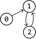
Consider a simple case where there are just two courses. A scenario where enrollment into all courses is impossible occurs when each course is a prerequisite to the other, as graphically represented below:

Here are a couple of impossible enrollment scenarios that could occur with prerequisites for three courses:

What do we notice about these cases and their graphical representations? They both have a circular relationship: a cycle. This highlights that it’s impossible to enroll in all courses if there exists a circular dependency between courses. In other words, there must not be a cycle in the graphical representation of the courses for complete enrollment to be possible.

Another thing to note is that the first courses which can be completed are those without prerequisites. In the graphical representation, such a course would have no directed arrows pointing at them. Let’s refer to the number of directed edges incoming to a node as the in-degree of that node.

In the example below, each node's in-degree is displayed at the top right:

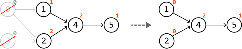
Courses 0 and 3 have an in-degree of 0. So, let’s complete them first and remove them from the graph. By doing this, we reduce the number of prerequisites for courses 1 and 2. Course 1's indegree then decreases by 1, and course 2's indegree decreases by 2:

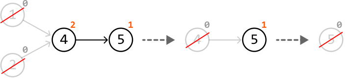
Now, courses 1 and 2 have an in-degree of 0, which means we can enroll in them and remove them from the graph. Observe what happens when we continue the process of removing courses with an in-degree of 0 from the graph:

By the end of this process, no courses remain, indicating it’s possible to enroll in all courses.

Now, consider an example with a cyclic dependency:

Let's follow the same steps of removing courses with an in-degree of 0:

Here, there is no way to progress because there aren't any courses with an in-degree of 0. When this happens, and there are still unvisited courses, a cyclic dependency exists, meaning enrolment is impossible.

Now, let’s identify a way to simulate the above process algorithmically.

Topological sort
The process we described above is essentially topological sorting, where vertices of a graph are sorted in such a way that for every directed edge u → v, node u comes before node v in the ordering of the topological sort.

An algorithm designed to perform topological sort is Kahn’s algorithm. Let’s see how we can use it to solve this problem.

The first step of Kahn's algorithm is to determine the in-degree of each course. This can be achieved by counting the number of times each course appears as a dependent in the prerequisite pairs: for a pair [a, b], course b depends on course a, so course b’s in-degree is incremented by one:

Now, we want to process all the courses with an in-degree of 0 first. We can add these courses to a queue to be processed:

To begin processing, pop the first course from the queue: course 0. Then, for each course that has course 0 as a prerequisite (i.e., courses pointed to by course 0), reduce their in-degree by one:

If any of the courses have an in-degree of 0 after being decremented, add them to the queue. Course 1 now has an in-degree of 0, so we add it to the queue:

We can continue the above process until the queue is empty, indicating that there aren't any more courses with an in-degree of 0.

• If we've processed all n courses, enrollment to all courses is possible.
• If we couldn’t process all n courses, a cycle was found, indicating enrollment to all courses is impossible.

Implementation

from typing import List
from collections import defaultdict, deque
    
def prerequisites(n: int, prerequisites: List[List[int]]) -> bool:
    graph = defaultdict(list)
    in_degrees = [0] * n
    # Represent the graph as an adjacency list and record the in-degree of each
    # course.
    for prerequisite, course in prerequisites:
        graph[prerequisite].append(course)
        in_degrees[course] += 1
    queue = deque()
    # Add all courses with an in-degree of 0 to the queue.
    for i in range(n):
        if in_degrees[i] == 0:
            queue.append(i)
    enrolled_courses = 0
    # Perform topological sort.
    while queue:
        node = queue.popleft()
        enrolled_courses += 1
        for neighbor in graph[node]:
            in_degrees[neighbor] -= 1
            # If the in-degree of a neighboring course becomes 0, add it to the queue.
            if in_degrees[neighbor] == 0:
                queue.append(neighbor)
    # Return true if we've successfully enrolled in all courses.
    return enrolled_courses == n

#include <vector>
#include <queue>
using namespace std;

bool prerequisites(int n, vector<vector<int>>& edges) {
    vector<vector<int>> graph(n);
    vector<int> indegree(n, 0);
    for (int i = 0; i < (int)edges.size(); i++) {
        int a = edges[i][0];
        int b = edges[i][1];
        graph[a].push_back(b);           // a before b
        indegree[b]++;
    }
    queue<int> q;
    for (int i = 0; i < n; i++) {
        if (indegree[i] == 0) {
            q.push(i);
        }
    }
    int taken = 0;
    while (!q.empty()) {
        int course = q.front();
        q.pop();
        taken++;
        for (int b : graph[course]) {
            indegree[b]--;               // one prerequisite satisfied
            if (indegree[b] == 0) {
                q.push(b);               // now ready to take
            }
        }
    }
    return taken == n;
}

boolean prerequisites(int n, int[][] edges) {
    List<List<Integer>> graph = new ArrayList<>();
    for (int i = 0; i < n; i++) {
        graph.add(new ArrayList<>());
    }
    int[] indegree = new int[n];
    for (int[] e : edges) {
        graph.get(e[0]).add(e[1]);       // a before b
        indegree[e[1]]++;
    }
    Queue<Integer> q = new LinkedList<>();
    for (int i = 0; i < n; i++) {
        if (indegree[i] == 0) {
            q.add(i);
        }
    }
    int taken = 0;
    while (!q.isEmpty()) {
        int course = q.poll();
        taken++;
        for (int b : graph.get(course)) {
            indegree[b]--;               // one prerequisite satisfied
            if (indegree[b] == 0) {
                q.add(b);                // now ready to take
            }
        }
    }
    return taken == n;
}

Complexity Analysis

Time complexity: The time complexity of prerequisites is $O(n+e)$ where $e$ denotes the number of edges derived from the prerequisites array. Here’s why:

• Creating the adjacency list and recording the in-degrees takes $O(e)$ time because we iterate through each prerequisite once.

• Adding all courses with in-degree 0 to the queue takes $O(n)$ time because we check the in-degree of each course once.

• Performing Kahn’s algorithm takes $O(n+e)$ time because each course and prerequisite is processed at most once during the traversal.

Space complexity: The space complexity is $O(n+e)$, since the adjacency list takes up $O(n+e)$ space, while the in_degrees array and queue each take up $O(n)$ space.

Dry Runs

Two step-by-step walkthroughs of the algorithm below: a valid case (the expected happy path) and an invalid / edge case that exercises the tricky parts. Each step shows the program state as the code runs—the same steps apply to Python, C++ and Java.

The same steps in each language