
Given two words, start and end, and a dictionary containing an array of words, return the length of the shortest transformation sequence to transform start to end. A transformation sequence is a series of words in which:
If no such transformation sequence exists, return 0.
Input: start = 'red', end = 'hit',
       dictionary = [
            'red', 'bed', 'hat', 'rod', 'rad', 'rat', 'hit', 'bad', 'bat'
       ]
Output: 5
New to this one? Start here. Below is the core idea in everyday language, plus a real-world analogy—then the sections that follow build on it with the formal reasoning, code, and step-by-step walkthroughs.
Each dictionary word is a stone, and two stones are joined if they differ by exactly one letter. You must hop from start to end in the fewest hops. Fewest-hops on an unweighted map of connections is the textbook job of BFS: explore all words one hop away, then all words two hops away, and so on — the first time you touch end, you have used the shortest ladder.
In a transformation sequence, each transformation involves changing one letter of a word to get another word. Consider the following example:
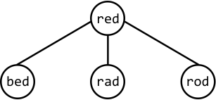
We know our transformation sequence should start with the word “red”, but how can we identify subsequent words in the sequence? The words that could immediately follow “red” are “bed”, “rad”, or “rod”, since each differs from “red” by one letter:
Similarly, we can make a direct connection between each word and its one-letter-off neighbors:
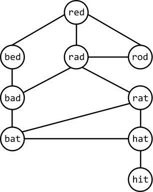
This structure resembles a graph, indicating that finding the shortest transformation sequence involves finding the shortest path in this graph from the start node (“red”) to the end node (“hit”):
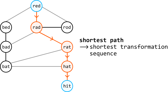
Finding the shortest path
When tasked with a graph problem that involves finding the shortest path between two nodes, BFS should come to mind. From the start node, BFS works by exploring all neighbors at a distance of 1 from the start node, followed by exploring nodes at a distance of 2, and so on. This means that once we find the end node, we’ve reached it via the shortest possible distance.
So, let’s use level-order traversal, a variant of BFS, to find the shortest path in this graph, where each level we traverse represents nodes that are a specific distance from the start node:
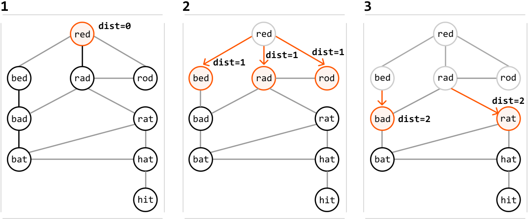
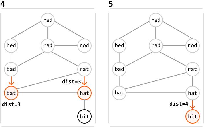
As we can see, we managed to find the end node via the shortest path. To return the length of this path, we return dist, plus 1, to include the start node. If you’re unfamiliar with how level-order traversal works, review the Matrix Infection problem in this chapter.
Note that during traversal, we need to ensure we don’t revisit previously traversed strings. By storing the visited strings in a hash set, we can quickly check if a string was already visited.
Now, let’s figure out how to build the above graph.
Building the graph
We can represent the graph as an adjacency list, where each word has a list of all of its neighboring words:
![Image represents a graph data structure depicted in a textual format. The text is labeled 'graph:' and presents a series of key-value pairs. Each key is a string enclosed in double quotes (e.g., 'red'), representing a node in the graph. The value associated with each key is a list of strings, also enclosed in square brackets, representing the nodes directly connected to the key node (its neighbors). For instance, 'red': [ 'bed', 'rad', 'rod'] indicates that the node 'red' is connected to nodes 'bed', 'rad', and 'rod'. Similarly, 'bed' connects to 'red' and 'bad', 'hat' connects to 'rat', 'bat', and 'hit', and 'hit' connects only to 'hat'. The ellipsis (...) suggests that there might be more key-value pairs not shown in the image, implying a larger graph. The overall structure represents an adjacency list representation of a directed or undirected graph, depending on whether the connections are considered bidirectional.](images/img-8b88f9c4d77d.svg)
The challenge here is finding each word’s neighbors. Consider the word “red”. One way we can identify all words that are one letter different from “red” is to generate all possible words by changing each letter in “red” to every other letter in the alphabet. For each of these generated words, we check if it exists in the dictionary. If it does, it’s a neighbor of “red”:
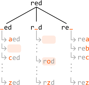
To make checking the dictionary more efficient, we can store the words from the dictionary in a hash set, enabling us to verify the existence of a word in constant time.
Note that before we build the graph, it’s important to check if start or end exists in the dictionary. If either is missing, we can immediately return 0, since each word in the sequence needs to be in the dictionary.
Space optimization
The purpose of the above adjacency list is to facilitate graph traversal. However, we can avoid building it altogether by leveraging the fact that each word in the dictionary is only visited once during the BFS traversal, indicating we only ever need access to the neighbors of each word once.
If we had a way to generate each word’s neighbors when needed during BFS traversal, we could avoid creating the adjacency list, and save some space that would otherwise be taken up by it.
def shortest_transformation_sequence(start: str, end: str, dictionary: List[str]) -> int:
    dictionary_set = set(dictionary)
    if start not in dictionary_set or end not in dictionary_set:
        return 0
    if start == end:
        return 1
    lower_case_alphabet = 'abcdefghijklmnopqrstuvwxyz'
    queue = deque([start])
    visited = set([start])
    dist = 0
    # Use level-order traversal to find the shortest path from the start word to the
    # end word.
    while queue:
        for _ in range(len(queue)):
            curr_word = queue.popleft()
            # If we found the end word, we've reached it via the shortest path.
            if curr_word == end:
                return dist + 1
            # Generate all possible words that have a one-letter difference to the
            # current word.
            for i in range(len(curr_word)):
                for c in lower_case_alphabet:
                    next_word = curr_word[:i] + c + curr_word[i+1:]
                    # If 'next_word' exists in the dictionary, it's a neighbor of the
                    # current word. If it's unvisited, add it to the queue to be
                    # processed in the next level.
                    if next_word in dictionary_set and next_word not in visited:
                        visited.add(next_word)
                        queue.append(next_word)
        dist += 1
    # If there is no way to reach the end node, then no path exists.
    return 0
#include <string>
#include <vector>
#include <queue>
#include <unordered_set>
using namespace std;
int shortestTransformationSequence(string start, string end, vector<string>& dictionary) {
unordered_set<string> wordSet(dictionary.begin(), dictionary.end());
if (wordSet.count(start) == 0 || wordSet.count(end) == 0) {
return 0;
}
if (start == end) {
return 1;
}
queue<pair<string, int>> q;
q.push({start, 1});
unordered_set<string> visited;
visited.insert(start);
while (!q.empty()) {
pair<string, int> front = q.front();
q.pop();
string word = front.first;
int length = front.second;
for (int i = 0; i < (int)word.size(); i++) {
string next = word;
for (char ch = 'a'; ch <= 'z'; ch++) {
if (ch == word[i]) {
continue;
}
next[i] = ch;
if (next == end) {
return length + 1; // first time we reach end = shortest
}
if (wordSet.count(next) == 1 && visited.count(next) == 0) {
visited.insert(next);
q.push({next, length + 1});
}
}
}
}
return 0;
}int shortestTransformationSequence(String start, String end, List<String> dictionary) {
Set<String> wordSet = new HashSet<>(dictionary);
if (!wordSet.contains(start) || !wordSet.contains(end)) {
return 0;
}
if (start.equals(end)) {
return 1;
}
Queue<Object[]> q = new LinkedList<>();
q.add(new Object[]{start, 1});
Set<String> visited = new HashSet<>();
visited.add(start);
while (!q.isEmpty()) {
Object[] front = q.poll();
String word = (String) front[0];
int length = (int) front[1];
char[] chars = word.toCharArray();
for (int i = 0; i < chars.length; i++) {
char original = chars[i];
for (char ch = 'a'; ch <= 'z'; ch++) {
if (ch == original) {
continue;
}
chars[i] = ch;
String next = new String(chars);
if (next.equals(end)) {
return length + 1; // first time we reach end = shortest
}
if (wordSet.contains(next) && !visited.contains(next)) {
visited.add(next);
q.add(new Object[]{next, length + 1});
}
}
chars[i] = original;
}
}
return 0;
}Time complexity: The time complexity of shortest_transformation_sequence is , where denotes the number of words in the dictionary, and denotes the length of a word. Here’s why:
Creating a hash set containing all the words in the dictionary takes time, because hashing each of the words takes time.
Level-order traversal processes at most words from the dictionary. At each of these words, we generate up to transformations, and it takes time to check if a transformation exists in the visited and dictionary_set hash sets, and to enqueue it. This means level-order traversal takes approximately time.
Therefore, the overall time complexity is .
Space complexity: The space complexity is , taken up by the dictionary_set hash set, the visited hash set, and the queue.
An important observation is that we don’t necessarily need to begin level-order traversal at the start word: we can also start a search at the end word. In fact, we can combine these by performing them simultaneously to find the shortest path. This is known as bidirectional BFS, or in this case, bidirectional level-order traversal.
When we perform two searches, one from start and one from end, the idea is that they will meet in the middle if a path between these two words exists. If a path doesn’t exist, the searches will never meet, indicating that a transformation sequence does not exist.
This optimization allows us to identify the shortest distance more quickly. We can see in the example below that regular level-order traversal ends up traversing through more nodes than in the bidirectional traversal, while also requiring 4 iterations instead of 2.
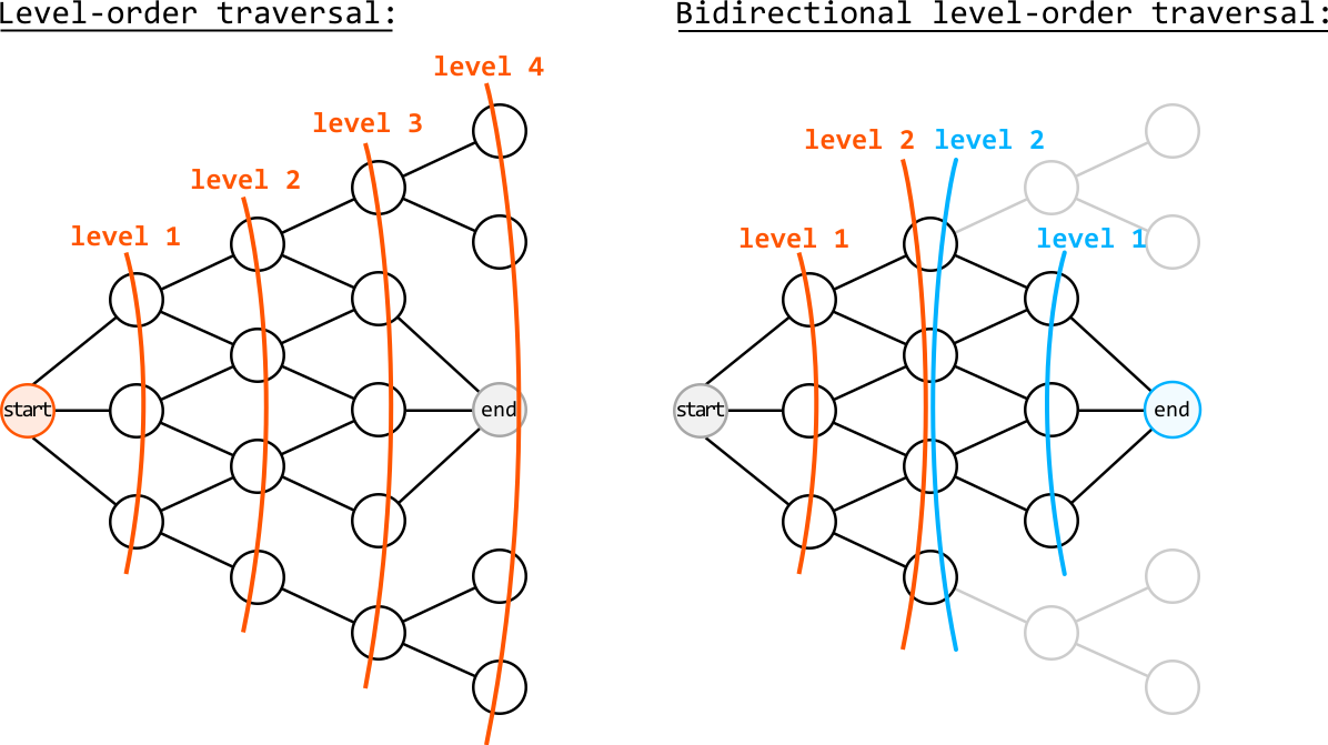
To simulate this process, we alternate between the two level-order traversals and progress through each search one level at a time:
We alternate between these two steps until a node visited in one search has already been visited in the other search, indicating that the traversals have met. Here’s what this alternating process looks like:
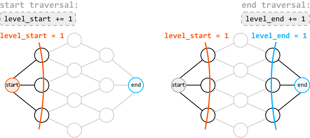
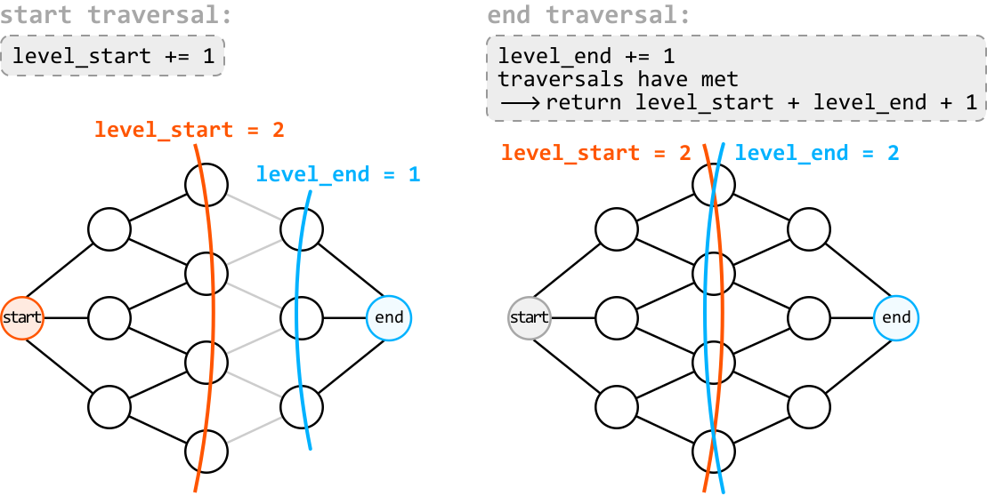
To check if a node has already been visited by the other traversal, we can query the visited hash set used by the other traversal. If a word exists in the visited hash set of the other traversal, we know the searches have met.
from typing import List
from collections import deque

def shortest_transformation_sequence_optimized(start: str, end: str, dictionary: List[str]) -> int:
    dictionary_set = set(dictionary)
    if start not in dictionary_set or end not in dictionary_set:
        return 0
    if start == end:
        return 1
    start_queue = deque([start])
    start_visited = {start}
    end_queue = deque([end])
    end_visited = {end}
    level_start = level_end = 0
    # Perform a level-order traversal from the start word and another from the end
    # word.
    while start_queue and end_queue:
        # Explore the next level of the traversal that starts from the start word. If
        # it meets the other traversal, the shortest path between 'start' and 'end'
        # has been found.
        level_start += 1
        if explore_level(start_queue, start_visited, end_visited, dictionary_set):
            return level_start + level_end + 1
        # Explore the next level of the traversal that starts from the end word.
        level_end += 1
        if explore_level(end_queue, end_visited, start_visited, dictionary_set):
            return level_start + level_end + 1
    # If the traversals never met, then no path exists.
    return 0

# This function explores the next level in the level-order traversal and checks if
# two searches meet.
def explore_level(queue, visited, other_visited, dictionary_set) -> bool:
    lower_case_alphabet = 'abcdefghijklmnopqrstuvwxyz'
    for _ in range(len(queue)):
        current_word = queue.popleft()
        for i in range(len(current_word)):
            for c in lower_case_alphabet:
                next_word = current_word[:i] + c + current_word[i+1:]
                # If 'next_word' has been visited during the other traversal, it means
                # both searches have met.
                if next_word in other_visited:
                    return True
                if next_word in dictionary_set and next_word not in visited:
                    visited.add(next_word)
                    queue.append(next_word)
    # If no word has been visited by the other traversal, the searches have not met
    # yet.
return FalseTime complexity: The time complexity of shortest_transformation_sequence_optimized is , since we’re performing two level-order traversals. Note that this is more efficient in practice since there are potentially fewer nodes to traverse when using bidirectional traversal.
Space complexity: The space complexity is , taken up by the dictionary_set hash set, the visited hash sets, and both queues.
Two step-by-step walkthroughs of the algorithm below: a valid case (the expected happy path) and an invalid / edge case that exercises the tricky parts. Each step shows the program state as the code runs—the same steps apply to Python, C++ and Java.
dictionary = [red, bed, hat, rod, rad, rat, hit, bad, bat]. BFS explores one layer (hop) at a time, left to right. Green = the layer just discovered, faded = not reached yet; the green path is the shortest ladder.
red at length 1 — the only word in the queue.
red and enqueue every dictionary word one letter away: rad, rod, bed.
rad we reach the new words rat and bad.
rat we reach hat and bat.
hat produces hit = end. First arrival is the shortest → return 5 (the green path).
| pop | length | new neighbors enqueued |
|---|---|---|
| red | 1 | rad, rod, bed (length 2) |
| rad | 2 | rat, bad (length 3) |
| rat | 3 | hat, bat (length 4) |
| hat | 4 | changes to hit == end → return 4 + 1 = 5 |
BFS reaches end the moment the shortest ladder completes → 5. ✓
start = "cat", end = "dog", dictionary = [cat, cog, dog]. Both are in the dictionary, but cat is 2+ letters from every other word — no edge connects them.
cat and generate every one-letter edit (patterns _at, c_t, ca_). None of them spell cog or dog — both differ by 2+ letters, so there is no edge out of cat.
end (dog, red) was never produced → return 0.
| pop | length | neighbors in dictionary |
|---|---|---|
| cat | 1 | none (cog, dog differ by 2+ letters) |
| — | — | queue empty, end never reached → return 0 |
A word ladder needs a chain of single-letter steps; a gap of two letters with no bridge word breaks it. ✗
Neighbors come from slicing: word[:i] + ch + word[i+1:]. The queue holds (word, length) tuples; visited is a set of strings.
Same steps. Copy the word, set one character, and compare. unordered_set<string> gives O(1) membership; the queue holds pair<string,int>.
Same steps. Edit a char[] and rebuild the String, then restore the character. Use .equals for word comparison, never ==.