Return the width of the widest level in a binary tree, where the width of a level is defined as the distance between its leftmost and rightmost non-null nodes.
Example:
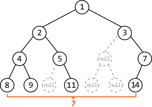
Output: 7
Return the width of the widest level in a binary tree, where the width of a level is defined as the distance between its leftmost and rightmost non-null nodes.
Output: 7
New to this one? Start here. Below is the core idea in everyday language, plus a real-world analogy—then the sections that follow build on it with the formal reasoning, code, and step-by-step walkthroughs.
Think of each level as a row of numbered theatre seats in a complete tree. The width is how many seats stretch from the leftmost occupied seat to the rightmost occupied one — empty seats in between still count toward the span (you still had to walk past them).
Let's first understand how width is defined in a binary tree. An important distinction to make is that the width of a level is not necessarily equivalent to the number of nodes in that level.
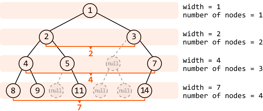
As we can see, the null nodes between the leftmost and rightmost nodes are considered in the width, as well.
Think about a data structure in which determining the width or distance between two elements is simple, such as an array, where the distance of two elements can be obtained by the difference between their indexes. If our binary tree also has indexes, it would similarly be possible to obtain the width between two nodes at a level. Let’s explore a method to assign an index to each node.
Indexing a binary tree
Below, we see how indexes can be assigned at each node, starting with index 0 for the root node:
![Image represents a binary tree structure visualized across multiple horizontal layers, each representing a level of the tree. The nodes of the tree are circles containing numbers (1, 2, 3, 4, 5, 7, 8, 9, 11, 14), with orange numbers next to them indicating a sequential node numbering. Solid lines connect parent nodes to their children, illustrating the hierarchical relationships. Dashed lines and circles labeled '[null]' represent missing nodes or branches. To the right of the tree, calculations are shown for 'width' at each level. The formula used is `width = (largest node index - smallest node index) + 1`, with the result displayed below. For example, at the lowest level, the calculation is `width = (13 - 7) + 1 = 7`, reflecting the number of nodes (including nulls) present at that level. The top level has a width of 1, the second level has a width of 2, the third level has a width of 4, and the bottom level has a width of 7.](images/img-1a529bbb36b9.svg)
These indexes enable us to calculate the width of a level using rightmost_index - leftmost_index + 1, as shown in the diagram above. Note, the indexes at the null nodes are added only for visualization.
But how can we set up something like this? The key observation is that each node's index can be determined from its parent's index. We can derive the following relationship for any node at index i:
2*i + 1.2*i + 2.Now, we just need a way to traverse each level of the tree to determine the width at individual levels, allowing us to obtain the width of the widest level in the tree. We can use level-order traversal for this.
Level-order traversal
If you're unfamiliar with the level-order traversal algorithm, study the Rightmost Nodes of a Binary Tree problem before continuing.
Remember, level-order traversal utilizes a queue to process the binary tree nodes. In this problem, whenever we push a node into this queue, we also push its respective index along with it, to know which index it’s associated with.
The width of a level can be calculated using rightmost_index - leftmost_index + 1. To perform this calculation, we need the index of the first (leftmost) and last (rightmost) nodes of that level. Here’s how we obtain these indexes:
Set leftmost_index to the index at the first node of the level.
Start rightmost_index at the same point as leftmost_index and update it as we traverse the level. This way, it will eventually be set to the last index after traversing the level.
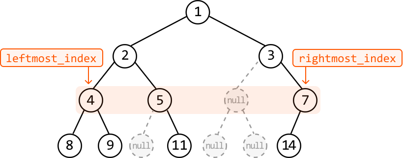
As we calculate the width at each level, we keep track of the largest width using max_width, representing the width of the widest level in the binary tree.
from ds import TreeNode

def widest_binary_tree_level(root: TreeNode) -> int:
    if not root:
        return 0
    max_width = 0
    queue = deque([(root, 0)])  # Stores (node, index) pairs.
    while queue:
        level_size = len(queue)
        # Set the 'leftmost_index' to the index of the first node in this level. Start
        # 'rightmost_index' at the same point as 'leftmost_index' and update it as we
        # traverse the level, eventually positioning it at the last node.
        leftmost_index = queue[0][1]
        rightmost_index = leftmost_index
        # Process all nodes at the current level.
        for _ in range(level_size):
            node, i = queue.popleft()
            if node.left:
                queue.append((node.left, 2*i + 1))
            if node.right:
                queue.append((node.right, 2*i + 2))
            rightmost_index = i
        max_width = max(max_width, rightmost_index - leftmost_index + 1)
    return max_width
int widestBinaryTreeLevel(TreeNode* root) {
if (root == nullptr) {
return 0;
}
long long best = 0;
queue<pair<TreeNode*, long long>> q;
q.push({root, 0});
while (!q.empty()) {
int sz = q.size();
long long first = q.front().second;
long long last = first;
for (int i = 0; i < sz; i++) {
auto [node, pos] = q.front();
q.pop();
long long index = pos - first; // normalize
last = index;
if (node->left != nullptr) {
q.push({node->left, 2 * index});
}
if (node->right != nullptr) {
q.push({node->right, 2 * index + 1});
}
}
best = max(best, last + 1);
}
return (int)best;
}int widestBinaryTreeLevel(TreeNode root) {
if (root == null) return 0;
long best = 0;
Queue<TreeNode> nodes = new LinkedList<>();
Queue<Long> pos = new LinkedList<>();
nodes.add(root); pos.add(0L);
while (!nodes.isEmpty()) {
int sz = nodes.size();
long first = pos.peek(), last = first;
for (int i = 0; i < sz; i++) {
TreeNode node = nodes.poll();
long index = pos.poll() - first; // normalize
last = index;
if (node.left != null) { nodes.add(node.left); pos.add(2 * index); }
if (node.right != null) { nodes.add(node.right); pos.add(2 * index + 1); }
}
best = Math.max(best, last + 1);
}
return (int) best;
}Time complexity: The time complexity of widest_binary_tree_level is , where denotes the number of nodes in the tree. This is because we process each node once during level-order traversal.
Space complexity: The space complexity is due to the space taken up by the queue. The queue’s size will grow as large as the level with the most nodes. In the worst case, this occurs at the last level when all the last-level nodes are non-null, totaling approximately nodes.
Two step-by-step walkthroughs of the algorithm below: a valid case (the expected happy path) and an invalid / edge case that exercises the tricky parts. Each step shows the program state as the code runs—the same steps apply to Python, C++ and Java.
| level | (node, position) | first | last | width = last−first+1 |
|---|---|---|---|---|
| 0 | (1, 0) | 0 | 0 | 1 |
| 1 | (3, 0), (2, 1) | 0 | 1 | 2 |
| 2 | (5, 0), (9, 3) | 0 | 3 | 4 |
On level 2, node 5 sits at position 0 and node 9 at position 3 (it is a right-child-of-a-right-child). The two empty slots between them count, so width = 4. answer = 4 ✓
| level | raw position would be | after subtracting first | width |
|---|---|---|---|
| 0 | 0 | 0 | 1 |
| 1 | 1 | 0 | 1 |
| 2 | 3 | 0 | 1 |
| … deep | 7, 15, 31, … (explodes) | 0 | 1 |
Each level has one node, so width is always 1. Without index -= first_index, the raw positions 0, 1, 3, 7, 15… would overflow a 32-bit int on a deep tree. Normalizing snaps the lone node back to position 0 every level, keeping the math safe. answer = 1 ✓
Python integers never overflow, so normalization is about keeping numbers small and readable here — but it makes the logic identical across languages.
Positions are long long and we still normalize, because even 64 bits overflow eventually on a very deep tree. Structured bindings auto [node, pos] unpack the pair.
Two parallel queues (nodes and pos) keep it simple; positions are Long. Normalizing is what makes 32-bit-ish trees safe.